Pairwise summation of numbers
Primary authors of this description: A.V.Frolov, Vad.V.Voevodin (Section 2.2), A.M.Teplov (Section 2.4)
Contents
- 1 Properties and structure of the algorithm
- 1.1 General description of the algorithm
- 1.2 Mathematical description of the algorithm
- 1.3 Computational kernel of the algorithm
- 1.4 Macro structure of the algorithm
- 1.5 Implementation scheme of the serial algorithm
- 1.6 Serial complexity of the algorithm
- 1.7 Information graph
- 1.8 Parallelization resource of the algorithm
- 1.9 Input and output data of the algorithm
- 1.10 Properties of the algorithm
- 2 Software implementation of the algorithm
- 3 References
1 Properties and structure of the algorithm
1.1 General description of the algorithm
The technique of pairwise execution is used to accelerate the calculation of long sequences of associative operations (for instance, mass summations). It is widely used because of its computational characteristics and the fact that the height of this algorithm is minimum possible. Its popularity among the non-numerical algorithms is related to its recursive nature, which simplifies its formulation.
1.2 Mathematical description of the algorithm
Input data: one-dimensional numeric array of size [math]n[/math].
Output data: sum of the array's elements.
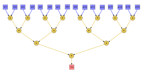
Formulas of the method: At each stage, the current array is first partitioned into pairs, and then the elements in each pair are summed. The resulting sums (and the elements not used at this stage) form an array that is partitioned into pairs at the next stage, etc.
1.3 Computational kernel of the algorithm
The computational kernel of the serial-parallel summation method can be compiled either of elementary pairwise additions (there are on the whole [math]n - 1[/math] additions) or in a recursive manner, that is, as a set of implementations of the pairwise summation for shorter arrays.
1.4 Macro structure of the algorithm
As already noted in the description of the computational kernel, the basic part of the method is compiled of recursive calls of the summation procedure for shorter arrays.
1.5 Implementation scheme of the serial algorithm
In its pure form, the pairwise summation is rarely used in a serial implementation because this complicates the general scheme of the algorithm and sharply increases the size of memory for storing intermediate data.
1.6 Serial complexity of the algorithm
Various ways of summation of an array of size [math]n[/math] differ from each other only by the arrangement of parentheses in the sum. The number of additions is the same for all arrangements, namely, [math]n - 1[/math]. Thus, in terms of serial complexity, the method should be qualified as a linear complexity algorithm.
1.7 Information graph
The algorithm graph is shown in the fig.1 in the case where an array of size 16 is summed. The vertices corresponding to the input data are depicted in blue, while those that correspond to output data are depicted in red.
1.8 Parallelization resource of the algorithm
The parallel version of the pairwise summation for an array of size [math]n[/math] requires that [math]\lceil \log_2 n \rceil[/math] layers be successively performed. The number of additions per layer decreases from [math]\frac{n}{2}[/math] to [math]1[/math]). In terms of the parallel form height, the pairwise summation is qualified as a logarithmic complexity algorithm. Its complexity is linear in terms of the parallel form width.
1.9 Input and output data of the algorithm
Input data: array [math]x[/math] (with elements [math]x_i[/math]).
Further restrictions: none.
Size of the input data: [math]N[/math].
Output data: sum of the array's elements.
Size of the output data: single scalar.
1.10 Properties of the algorithm
It is clear that, in the case of unlimited resources, the ratio of the serial to parallel complexity has the order [math]\frac{n}{\log_2 n}[/math] (the ratio of the linear to logarithmic complexity). The computational power of the algorithm, understood as the ratio of the number of operations to the total size of the input and output data, is only 1 (the size of the input and output data is almost equal to the number of operations). The algorithm is completely determined. The edges of the information graph are nonlocal. For any placing of graph vertices, the length of the edges grows exponentially from a layer to the next layer.
