Bellman-Ford, locality
Primary author of this description: I.V.Afanasyev.
Contents
1 Links
The basic fragment of the implementation used for obtaining quantitative estimates is given here (function Kernel).
2 Locality of data and computations
2.1 Locality of implementation
2.1.1 Structure of memory access and a qualitative estimation of locality
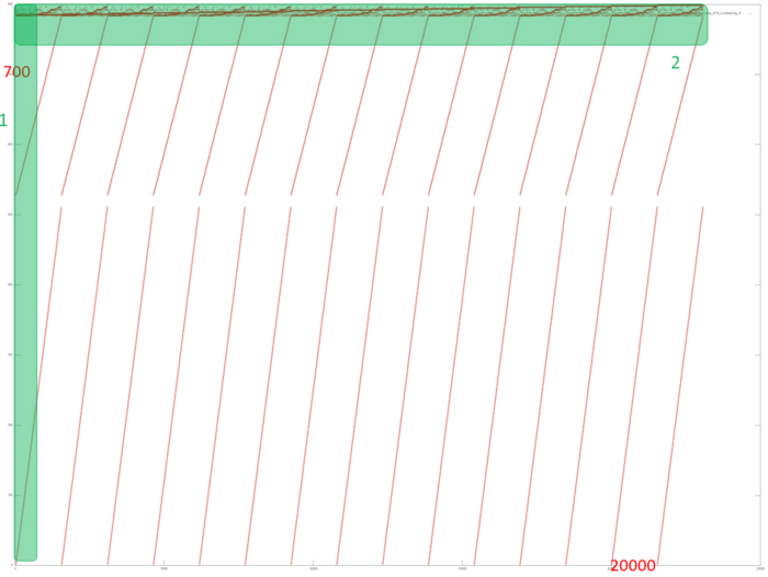
Fig.1 shows the memory access profile for an implementation of the Bellman-Ford algorithm. The first thing that should be noted is that the number of memory accesses is much greater than the number of involved data. This says that the data are often used repeatedly, which usually implies high temporal locality. Furthermore, it is evident that the memory accesses have an explicit regular structure; one can also see repeated iterations in the work of the algorithm. Practically all the accesses form fragments similar to a successive search. The upper part of the figure, where the structure is more complicated, is an exception.
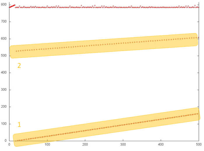
In order to better understand the structure of the overall profile, let us consider more closely its individual areas. Figure 2 shows fragment 1 (selected in fig.1); here, one can see the first 500 memory accesses (note that different slopes of two successive searches are caused by different ratios of sides in the corresponding areas). This figure shows that parts 1 and 2 (selected in yellow) are practically identical successive searches. They only differ in that the accesses in part 1 are performed twice as often compared to part 2; for this reason, the former is represented by a greater number of points. As is known, such profiles are characterized by high spatial and low temporal locality.
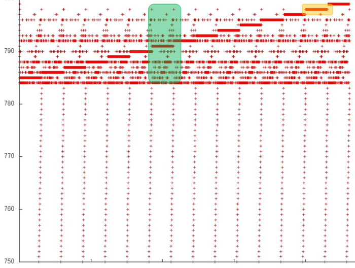
Now, we consider the more interesting fragment 2 of fig.1 (see fig.3). In the lower area of this profile, one can again see a confirmation of the regularity of accesses. However, its upper area is clearly structured in a more complex way, although the regularity is seen here as well. In particular, the same repeated iterations are present here; in them, one can distinguish long sequences of accesses to the same data. An example of such a behavior, which is optimal in terms of locality, is set out in yellow.
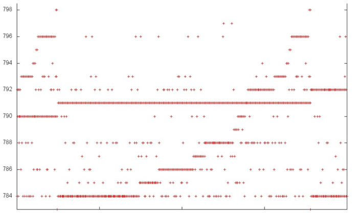
In order to understand the structure of memory accesses in the upper area, let us examine this area even more closely. Consider the visualization of the small portion of fragment 2 shown in green in fig.3. In this case, the closer examination (see fig.4) does not make the picture more clear: one can see an irregular structure within an iteration, but the nature of this irregularity is fairly difficult to describe. However, such a description is not required here. Indeed, one can notice that only 15 elements are located along the vertical, whereas the number of accesses to these elements is much greater. Such a profile has a very high locality (both spatial and temporal) regardless of the structure of accesses.
The majority of accesses are performed exactly to fragment 2. Consequently, one can state that the overall profile also has a high spatial and temporal locality.
2.1.2 Quantitative estimation of locality
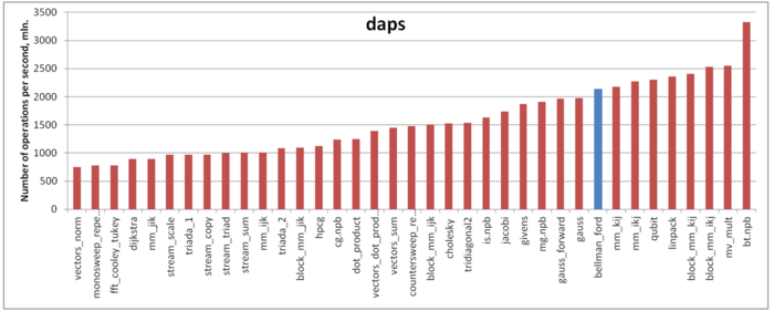
Our estimate is based on daps, which assesses the number of memory accesses (reads and writes) per second. Similarly to flops, daps is used to evaluate memory access performance rather than locality. Yet, it is a good source of information, particularly for comparison with the results provided by the estimate cvg.
Fig.5 shows daps values for implementations of popular algorithms, sorted in ascending order (the higher the daps, the better the performance in general). One can see that the memory access performance of this implementation is fairly good. In particular, its daps value is comparable with that for the Linpack benchmark. The latter is known for its high efficiency of memory interaction.
