Linpack, locality

Primary author of this description: Vad.V.Voevodin (Section 2).

1 Links

The basic fragment of the implementation used for obtaining quantitative estimates is given here (the original code is taken from here).

2 Locality of data and computations

2.1 Locality of implementation

2.1.1 Structure of memory access and a qualitative estimation of locality

Figure 1. Linpack benchmark. Overall memory access profile

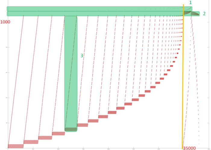
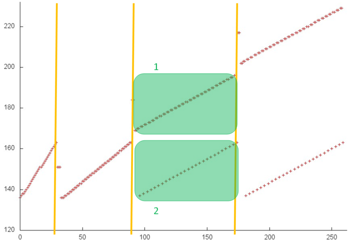
Fig.1 shows the overall memory address profile for the Linpack benchmark. Here, three arrays are used. In Fig.1, the accesses to the first two arrays are distinguished in green (fragments 1 and 2). The other accesses are performed to the entries of the third array, which contains the coefficient matrix of the SLAE. The test consists of two stages, namely, the factorization of the coefficient matrix and the subsequent solution of the SLAE. In figure, the stages are divided by the orange line. One can see that the first stage has an iterative structure, and several matrix entries with smallest indices are dropped from the analysis at each iteration step. One can also notice that the second stage performs two passes with an increasing step over the matrix entries; the first pass is direct, while the second goes in the reverse direction. On the whole, the profile has a fairly complex structure, and a more detailed analysis is needed to understand its locality properties.

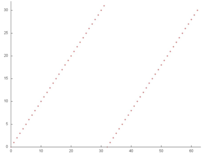
Fragment 1 is shown separately in Fig.2. The fragment is very small compared to the overall profile, but, with this proximity, it is easily seen that this fragment consists of two serial searches of all the array entries. Such a search is characterized by high spatial locality and rather low temporal locality because only two accesses to each entry are performed.

Figure 2. Fragment 1 (access profile for the first array)

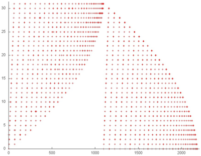
Now, we discuss fragment 2, which is shown in Fig.3. This profile consists of two similar stages; both are sets of iterations. At each iteration step, a serial search is performed, and one array entry is dropped from the analysis. This is the entry with the minimum index, at the first stage, and the entry with the maximum index, at the second stage.

Both the spatial and temporal localities of this profile are very high because the accesses are almost always made to nearby entries; moreover, the entries are fairly easy accessed repeatedly. However, note that this fragment consists of only about 2000 elements, which is considerably less than the overall number of accesses in the program. Consequently, the most of accesses (and, probably, the main impact) are due to the last array.

Figure 3. Fragment 2 (access profile for the second array)

Figure 4 shows fragment 3, selected from fig.1. This fragment depicts one iteration of the loop within which this array is accessed. It is easily seen from the figure that the iteration consists of two parts corresponding to two inner loops. The number of accesses at each iteration of both inner loops is about the same. However, at the next iteration, the first inner loop searches through the next portion of array entries, whereas the second searches through the same entries.

Figure 4. Fragment 3 (access profile for the third array, one iteration)

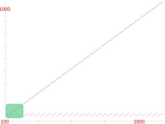
It remains to clarify the structure of memory accesses at the iterations of these two cycles. Consider in more detail the portion of fragment 3, which is shown in green in fig.4 (see fig.5).

Figure 5. Small portion of fragment 3, one iteration

One can see that the first two stages differ from the others because they execute certain initial operations. Then inner loops begin similar iterations; both perform serial searches of entries (see parts 1 and 2 shown in green). The basic difference is that two memory accesses per entry are done within the first loop.

The accesses to this array are characterized by a high spatial locality. Moreover, the second loop always uses the same entries, which also results in a rather high temporal locality. Thus, within one iteration (Fig.4), the locality of accesses is high. If accesses to the same entries are made at different iterations (and the number of accesses per iteration is not very large), then locality improves even further.

2.1.2 Quantitative estimation of locality

The launching conditions are described here.

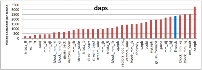
The first estimate is based on daps, which assesses the number of memory accesses (reads and writes) per second. Similar to flops, daps is used to evaluate memory access performance rather than locality. Yet, it is a good source of information, particularly for comparison with the results provided by the next estimate cvg.

Fig.6 shows daps values for implementations of popular algorithms, sorted in ascending order (the higher the daps, the better the performance in general). It is seen that the daps for the Linpack benchmark is among the highest values, which testifies to the efficiency of memory interaction.

Figure 6. Comparison of daps values

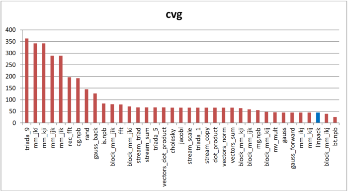
The second characteristic – cvg – is intended for obtaining a more machine-independent locality assessment. It determines how often a program needs to pull data to cache memory. Accordingly, the smaller the cvg value, the less frequently data need to be called to cache, and the better the locality.

Fig.7 shows the cvg values for the same set of implementations sorted in descending order (the smaller the cvg, the higher the locality in general). One can see that, according to this assessment, the locality of memory accesses for the Linpack benchmark is very high, which is consistent with earlier estimates and conclusions.

Figure 7. Comparison of cvg values