Linpack benchmark
Primary authors of this description: A.V.Frolov, Vad.V.Voevodin (Section 2.2), A.M.Teplov (раздел Section 2.4)
Contents
- 1 Properties and structure of the algorithm
- 1.1 General description of the algorithm
- 1.2 Mathematical description of the algorithm
- 1.3 Computational kernel of the algorithm
- 1.4 Macro structure of the algorithm
- 1.5 Implementation scheme of the serial algorithm
- 1.6 Serial complexity of the algorithm
- 1.7 Information graph
- 1.8 Parallelization resource of the algorithm
- 1.9 Input and output data of the algorithm
- 1.10 Properties of the algorithm
- 2 Software implementation of the algorithm
- 2.1 Implementation peculiarities of the serial algorithm
- 2.2 Locality of data and computations
- 2.3 Possible methods and considerations for parallel implementation of the algorithm
- 2.4 Scalability of the algorithm and its implementations
- 2.5 Dynamic characteristics and efficiency of the algorithm implementation
- 2.6 Conclusions for different classes of computer architecture
- 2.7 Existing implementations of the algorithm
- 3 References
1 Properties and structure of the algorithm
1.1 General description of the algorithm
Linpack benchmark is a test developed as a supplement to the Linpack library for testing the performance of computer systems. Actually, this test generates a system of linear algebraic equations (SLAE) [math]A \vec{x} = \vec{b}[/math] with a random dense square matrix [math]A[/math] and a vector [math]\vec{b}[/math] chosen so that the solution of the system is the vector [math]\vec{x}[/math] all of whose components are ones; then this SLAE is solved. In view of the general (with certain provisos) nature of the matrix, the solution of the system is divided into several stages. First, the [math]PLU[/math]-decomposition of [math]A[/math] is calculated by using Gaussian elimination with column pivoting ([math]P[/math] is a permutation matrix, [math]L[/math] is a lower triangular matrix with unit diagonal, and [math]U[/math] is an upper triangular matrix). At the second stage, the calculated decomposition is used to solve the SLAE [math]P L U \vec{x} = \vec{b}[/math]. At the third stage, the residual [math]\vec{r} = A \vec{x} - \vec{b}[/math] and the related characteristics are calculated. Then the data concerning the resulting accuracy and performance are produced. The performance is only estimated for the main part of the algorithm; that is, the calculations spent on the residual and norms are ignored.
The Linpack benchmark, which was developed for testing computers of traditional architecture, should not be confused with High Performance Linpack benchmark. The latter was devised for testing parallel computer systems and is based on a different (albeit similar) algorithm.
1.2 Mathematical description of the algorithm
Input data: square matrix [math]A[/math] (with entries [math]a_{ij}[/math]) (in 1992 version, the random number generator is chosen so that to ensure the non-singularity of [math]A[/math]), the right-hand side vector [math]\vec{b}[/math] (with components [math]b_i[/math]). Actually, they are not exactly input data (because the entries of the matrix are pseudo-random numbers generated by the program itself; these numbers are contained in the interval (-1/2, +1/2), and the right-hand sides are calculated as [math]b_i = \sum\limits_{j = 1}^i a_{ij}[/math]). However, in order to analyze the general scheme of the algorithm, it is convenient to regard [math]A[/math] and [math]\vec{b}[/math] as the input data.
Data to be calculated: lower triangular matrix [math]L[/math] (with entries [math]l_{ij}[/math]), upper triangular matrix [math]U[/math] (with entries [math]u_{ij}[/math]), permutation matrix [math]P[/math] (which is calculated as a collection of pivot indices rather than a full square array), and the solution vector [math]x[/math] (with components [math]x_i[/math]).
Here, we do not give detailed formulas of individual parts of the algorithm. These parts are independent algorithms, and their detailed descriptions should be presented separately. Consequently, we only discuss the general scheme of the algorithm.
The first part — decomposing the matrix into the product of two triangular matrices and a permutation matrix: [math]A = P L U[/math] — is performed by using Gaussian elimination with column pivoting. The permutation matrix is stored as a vector containing information on the performed permutations. The matrix [math]L[/math] is lower triangular with unit diagonal, while [math]U[/math] is an upper triangular matrix.
The second part is solving two triangular SLAEs. First, the system [math]L \vec{y} = P T \vec{b}[/math] is solved by forward substitution, then back substitution is used to solve the system [math]U \vec{x} = \vec{y}[/math]. This test stores both triangular matrices in the corresponding portions of the matrix [math]A[/math]. For this reason, [math]A[/math] is generated again (with the same starting parameters for the random number generator) before passing to the third part.
The third part (for which the performance is not measured) calculates first the residual of the solution [math]\vec{r} = A \vec{x} - \vec{b}[/math] and then its uniform norm, as well as the norm of the solution. On the completion of this stage, the algorithm outputs data related to the accuracy of the calculated solution and evaluates the performance of the system.
1.3 Computational kernel of the algorithm
The main part of the algorithm, which is the decomposition of a matrix via Gaussian elimination with column pivoting, is responsible for the bulk of operations. The second most important part is the calculation of the residual and its norm. It is implemented by the subroutine that calculates the sum of a vector and a matrix-vector product and by the function calculating the uniform norm. Less important parts are forward substitution in the Gauss method and back substitution in this method.
1.4 Macro structure of the algorithm
As already said in the description of the computational kernel of the algorithm, the decomposition of a matrix via Gaussian elimination with column pivoting is responsible for the bulk of operations. This decomposition is the first macro operation. It is followed by the forward substitution and, right away, by the back substitution. On the regeneration of the matrix, the next macro operation is calculating the residual for the solution of the SLAE, followed by the calculation the uniform norms of the residual and the solution.
1.5 Implementation scheme of the serial algorithm
The mathematical description of the algorithm was given above. The standard test calculates the triangular decomposition in-place, and the solutions to the triangular systems in the forward and back substitution are written to the locations of the right-hand sides. For this reason, on the calculation of the solution, the coefficient matrix and the right-hand side are regenerated for the subsequent calculation of the residual. As soon as the residual is calculated, its norm and the norm of the solution can be calculated in any order, which does not affect the algorithm and its results.
1.6 Serial complexity of the algorithm
Since the main part of the algorithm is the decomposition of a matrix via Gaussian elimination with column pivoting, the algorithm, as well as this decomposition, has cubical complexity. Other parts have quadratic complexity; consequently, they do not give a comparable contribution to the overall complexity of the algorithm.
1.7 Information graph
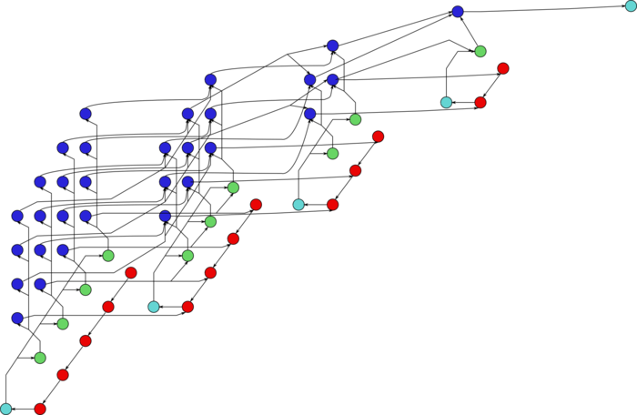
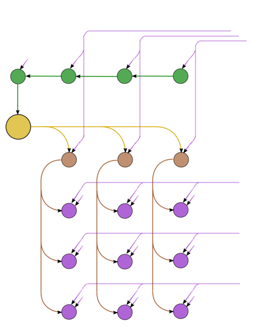
The graph consists of the information graphs of its basic parts. The first part (Gaussian elimination with column pivoting) has the most complex graph. Figure 1 shows the simplified graph of this part, post factum the choice of pivots. The operations of finding the maxima in the columns and saving the corresponding positions are given in green. The inversion of the current pivot, multiplications in the current column, and operations of the type [math]a b + c[/math] in the other columns are depicted in yellow, brown, and purple, respectively. Figure 2 shows the graph of a layer (one step of the method). The notation is the same as in the full graph. Dotted lines denote data communication from the pivot row.
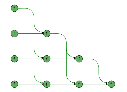
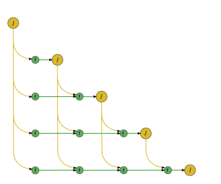
The second part consists of almost identical fragments. The first fragment describes the forward substitution, namely, the solution of the SLAE with a lower triangular matrix [math]L \vec{y} = \vec{b}[/math] (Fig.3). The diagonal entries of this matrix are ones; consequently, this fragment contains no divisions. All the green nodes correspond to the operations of the type [math]a b + c[/math]. The second fragment describes the back substitution, namely, the solution of the SLAE with an upper triangular matrix [math]U \vec{x} = \vec{y}[/math] (Fig.4). This matrix has no specific features; hence, the associated graph contains division operations, which are shown in yellow.
1.8 Parallelization resource of the algorithm
The analysis of parallelization resource of the algorithm shows that Gaussian elimination with column pivoting has the highest, namely, quadratic complexity (exactly because of the pivoting). The other parts of the algorithm have at most linear complexity. Therefore, to optimize calculations, the virtual researcher must optimize Gaussian elimination with column pivoting. Besides, the first fragment of the second part (that is, the solution of the first triangular SLAE) can be attached to the first part and executed almost entirely in the background of the latter. Indeed, both have the same direction of recalculating the data. However, the rest of the second part, despite its similarity to the first fragment, can only be executed on completion the latter. The reason is that these two fragments have opposite directions of recalculating the data.
1.9 Input and output data of the algorithm
Actually, this test has always the same data, which are calculated in the test itself. Consequently, in the strict sense, it has no input data.
The output data, produced by the test, are the norms of the residual, solution, and matrix, the ratios of these norms, and the computational power of the target computer system.
1.10 Properties of the algorithm
2 Software implementation of the algorithm
2.1 Implementation peculiarities of the serial algorithm
Strictly speaking, the investigator implementing the test for a computer system tests at the same time LINPAC or any other package from which procedures for triangular decomposition and solving a SLAE with the help of this decomposition are called. The web versions of the test can also be used for testing other implementations of the Gauss method. It was already noted above that the triangular decomposition of the original matrix is calculated in-place, and, in the course of forward and back substitution, the solutions are written to the locations of right-hand sides. This causes the necessity to regenerate both the coefficient matrix and the right-hand side for the subsequent calculation of the residual. This organization of the algorithm may well be changed in order to optimize the test.
2.2 Locality of data and computations
2.2.1 Locality of implementation
2.2.1.1 Structure of memory access and a qualitative estimation of locality
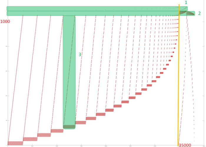
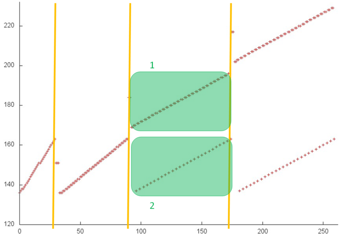
Fig.5 shows the overall memory address profile for the Linpack benchmark. Here, three arrays are used. In Fig.5, the accesses to the first two arrays are distinguished in green (fragments 1 and 2). The other accesses are performed to the entries of the third array, which contains the coefficient matrix of the SLAE. The test consists of two stages, namely, the factorization of the coefficient matrix and the subsequent solution of the SLAE. In figure, the stages are divided by the orange line. One can see that the first stage has an iterative structure, and several matrix entries with smallest indices are dropped from the analysis at each iteration step. One can also notice that the second stage performs two passes with an increasing step over the matrix entries; the first pass is direct, while the second goes in the reverse direction. On the whole, the profile has a fairly complex structure, and a more detailed analysis is needed to understand its locality properties.
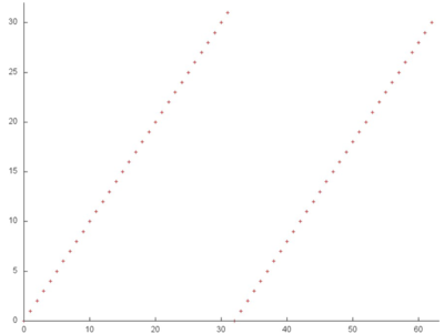
Fragment 1 is shown separately in Fig.6. The fragment is very small compared to the overall profile, but, with this proximity, it is easily seen that this fragment consists of two serial searches of all the array entries. Such a search is characterized by high spatial locality and rather low temporal locality because only two accesses to each entry are performed.
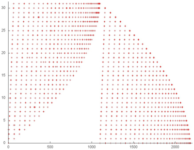
Now, we discuss fragment 2, which is shown in Fig.7. This profile consists of two similar stages; both are sets of iterations. At each iteration step, a serial search is performed, and one array entry is dropped from the analysis. This is the entry with the minimum index, at the first stage, and the entry with the maximum index, at the second stage.
Both the spatial and temporal localities of this profile are very high because the accesses are almost always made to nearby entries; moreover, the entries are fairly easy accessed repeatedly. However, note that this fragment consists of only about 2000 elements, which is considerably less than the overall number of accesses in the program. Consequently, the most of accesses (and, probably, the main impact) are due to the last array.
Figure 8 shows fragment 3, selected from fig.5. This fragment depicts one iteration of the loop within which this array is accessed. It is easily seen from the figure that the iteration consists of two parts corresponding to two inner loops. The number of accesses at each iteration of both inner loops is about the same. However, at the next iteration, the first inner loop searches through the next portion of array entries, whereas the second searches through the same entries.
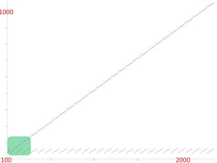
It remains to clarify the structure of memory accesses at the iterations of these two cycles. Consider in more detail the portion of fragment 3, which is shown in green in fig.8 (see fig.9).
One can see that the first two stages differ from the others because they execute certain initial operations. Then inner loops begin similar iterations; both perform serial searches of entries (see parts 1 and 2 shown in green). The basic difference is that two memory accesses per entry are done within the first loop.
The accesses to this array are characterized by a high spatial locality. Moreover, the second loop always uses the same entries, which also results in a rather high temporal locality. Thus, within one iteration (Fig.4), the locality of accesses is high. If accesses to the same entries are made at different iterations (and the number of accesses per iteration is not very large), then locality improves even further.
2.2.1.2 Quantitative estimation of locality
The basic fragment of the implementation used for obtaining quantitative estimates is given here (the original code is taken from here). The launching conditions are described here.
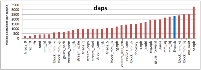
The first estimate is based on daps, which assesses the number of memory accesses (reads and writes) per second. Similar to flops, daps is used to evaluate memory access performance rather than locality. Yet, it is a good source of information, particularly for comparison with the results provided by the next estimate cvg.
Fig.10 shows daps values for implementations of popular algorithms, sorted in ascending order (the higher the daps, the better the performance in general). It is seen that the daps for the Linpack benchmark is among the highest values, which testifies to the efficiency of memory interaction.
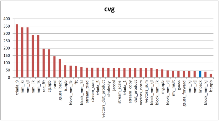
The second characteristic – cvg – is intended for obtaining a more machine-independent locality assessment. It determines how often a program needs to pull data to cache memory. Accordingly, the smaller the cvg value, the less frequently data need to be called to cache, and the better the locality.
Fig.11 shows the cvg values for the same set of implementations sorted in descending order (the smaller the cvg, the higher the locality in general). One can see that, according to this assessment, the locality of memory accesses for the Linpack benchmark is very high, which is consistent with earlier estimates and conclusions.
2.3 Possible methods and considerations for parallel implementation of the algorithm
2.4 Scalability of the algorithm and its implementations
2.4.1 Scalability of the algorithm
2.4.2 Scalability of of the algorithm implementation
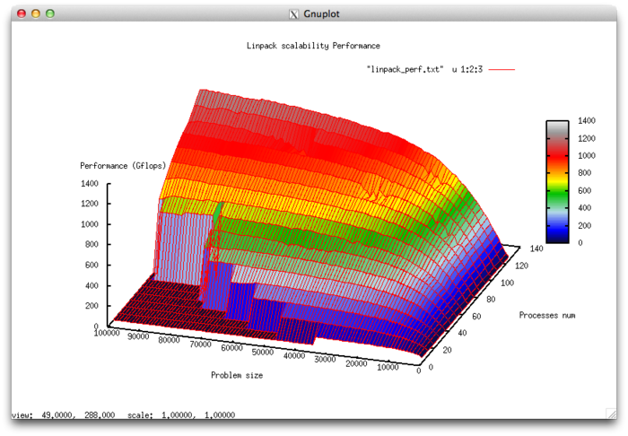
Let us study scalability for the implementation of the HPL Linpack test in accordance with Scalability methodology. This study was conducted using the Lomonosov supercomputer of the Moscow University Supercomputing Center.
Variable parameters for the launch of the algorithm implementation and the limits of parameter variations:
- number of processors [8 : 128] with the step 8;
- matrix size [1000 : 100000] with the step 1000.
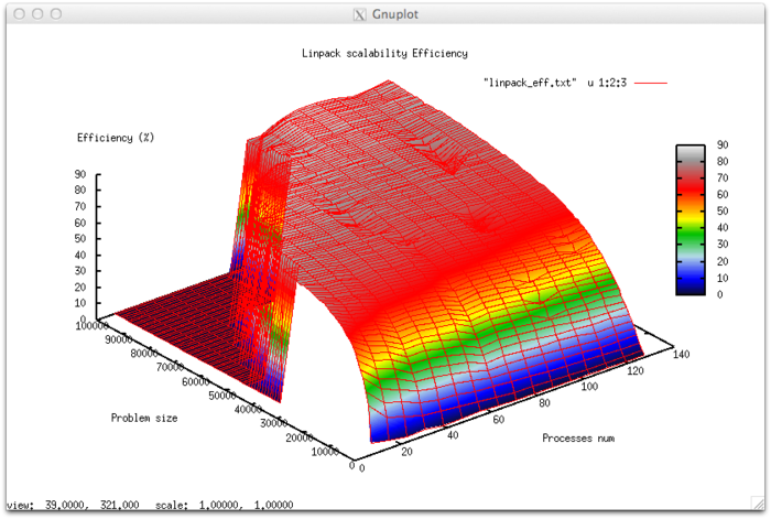
The experiments resulted in the following range of implementation efficiency:
- minimum implementation efficiency 0.039%;
- maximum implementation efficiency 86,7%.
The following figures show the graphs of the performance and efficiency for the HPL test as functions of the variable launch parameters.
Let us assess the scalability of the Linpack test:
- By the number of processes: -0.061256. As the number of processes increases, the efficiency (within the given range for the launch parameters) is reduced . But, overall, the reduction is not very rapid. The small intensity of the change is explained by the fact that, for large size problems, the overall efficiency is high. However, efficiency uniformly decreases with a rise in the number of processes. Another reason is that a rise in the computational complexity makes the reduction of efficiency not so fast. For the range covered, the decrease in the efficiency of the parallel program is explained by the growth of expenses on the organization of parallel execution. The reduction in efficiency is equally fast when the computational complexity increases and the number of processes is large. This confirms the surmise that the overhead expenses begin to strongly prevail over computations.
- By the size of a problem: 0.010134. Efficiency increases with the growth in the size of a problem. The increase is the faster the more processes are executed. This confirms the surmise that the problem size strongly affects the efficiency of execution. The estimate indicates that, within the given range for the launch parameters, efficiency markedly increases with the growth in the problem size. Taking into account that the difference between maximum and minimum efficiency is nearly 80 percent, we can also make the conclusion that the increase in efficiency regarded as a function of problem size is observed over the greater part of the range covered.
- Along two directions: 0.0000284. Suppose that both the computational complexity and the number of processes increase over the entire region under discussion. Then the efficiency increases; however, the increase in efficiency is not very significant.
Study of a test implementation
