Linpack benchmark

Primary authors of this description: A.V.Frolov, Vad.V.Voevodin (Section 2.2), A.M.Teplov (раздел Section 2.4)

1 Properties and structure of the algorithm

1.1 General description of the algorithm

Linpack benchmark is a test developed as a supplement to the Linpack library for testing the performance of computer systems. Actually, this test generates a system of linear algebraic equations (SLAE) [math]A \vec{x} = \vec{b}[/math] with a random dense square matrix [math]A[/math] and a vector [math]\vec{b}[/math] chosen so that the solution of the system is the vector [math]\vec{x}[/math] all of whose components are ones; then this SLAE is solved. In view of the general (with certain provisos) nature of the matrix, the solution of the system is divided into several stages. First, the [math]PLU[/math]-decomposition of [math]A[/math] is calculated by using Gaussian elimination with column pivoting ([math]P[/math] is a permutation matrix, [math]L[/math] is a lower triangular matrix with unit diagonal, and [math]U[/math] is an upper triangular matrix). At the second stage, the calculated decomposition is used to solve the SLAE [math]P L U \vec{x} = \vec{b}[/math]. At the third stage, the residual [math]\vec{r} = A \vec{x} - \vec{b}[/math] and the related characteristics are calculated. Then the data concerning the resulting accuracy and performance are produced. The performance is only estimated for the main part of the algorithm; that is, the calculations spent on the residual and norms are ignored.

The Linpack benchmark, which was developed for testing computers of traditional architecture, should not be confused with High Performance Linpack benchmark. The latter was devised for testing parallel computer systems and is based on a different (albeit similar) algorithm.

1.2 Mathematical description of the algorithm

Input data: square matrix [math]A[/math] (with entries [math]a_{ij}[/math]) (in 1992 version, the random number generator is chosen so that to ensure the non-singularity of [math]A[/math]), the right-hand side vector [math]\vec{b}[/math] (with components [math]b_i[/math]). Actually, they are not exactly input data (because the entries of the matrix are pseudo-random numbers generated by the program itself; these numbers are contained in the interval (-1/2, +1/2), and the right-hand sides are calculated as [math]b_i = \sum\limits_{j = 1}^i a_{ij}[/math]). However, in order to analyze the general scheme of the algorithm, it is convenient to regard [math]A[/math] and [math]\vec{b}[/math] as the input data.

Data to be calculated: lower triangular matrix [math]L[/math] (with entries [math]l_{ij}[/math]), upper triangular matrix [math]U[/math] (with entries [math]u_{ij}[/math]), permutation matrix [math]P[/math] (which is calculated as a collection of pivot indices rather than a full square array), and the solution vector [math]x[/math] (with components [math]x_i[/math]).

Here, we do not give detailed formulas of individual parts of the algorithm. These parts are independent algorithms, and their detailed descriptions should be presented separately. Consequently, we only discuss the general scheme of the algorithm.

The first part — decomposing the matrix into the product of two triangular matrices and a permutation matrix: [math]A = P L U[/math] — is performed by using Gaussian elimination with column pivoting. The permutation matrix is stored as a vector containing information on the performed permutations. The matrix [math]L[/math] is lower triangular with unit diagonal, while [math]U[/math] is an upper triangular matrix.

The second part is solving two triangular SLAEs. First, the system [math]L \vec{y} = P T \vec{b}[/math] is solved by forward substitution, then back substitution is used to solve the system [math]U \vec{x} = \vec{y}[/math]. This test stores both triangular matrices in the corresponding portions of the matrix [math]A[/math]. For this reason, [math]A[/math] is generated again (with the same starting parameters for the random number generator) before passing to the third part.

The third part (for which the performance is not measured) calculates first the residual of the solution [math]\vec{r} = A \vec{x} - \vec{b}[/math] and then its uniform norm, as well as the norm of the solution. On the completion of this stage, the algorithm outputs data related to the accuracy of the calculated solution and evaluates the performance of the system.

1.3 Computational kernel of the algorithm

The main part of the algorithm, which is the decomposition of a matrix via Gaussian elimination with column pivoting, is responsible for the bulk of operations. The second most important part is the calculation of the residual and its norm. It is implemented by the subroutine that calculates the sum of a vector and a matrix-vector product and by the function calculating the uniform norm. Less important parts are forward substitution in the Gauss method and back substitution in this method.

1.4 Macro structure of the algorithm

As already said in the description of the computational kernel of the algorithm, the decomposition of a matrix via Gaussian elimination with column pivoting is responsible for the bulk of operations. This decomposition is the first macro operation. It is followed by the forward substitution and, right away, by the back substitution. On the regeneration of the matrix, the next macro operation is calculating the residual for the solution of the SLAE, followed by the calculation the uniform norms of the residual and the solution.

1.5 Implementation scheme of the serial algorithm

The mathematical description of the algorithm was given above. The standard test calculates the triangular decomposition in-place, and the solutions to the triangular systems in the forward and back substitution are written to the locations of the right-hand sides. For this reason, on the calculation of the solution, the coefficient matrix and the right-hand side are regenerated for the subsequent calculation of the residual. As soon as the residual is calculated, its norm and the norm of the solution can be calculated in any order, which does not affect the algorithm and its results.

1.6 Serial complexity of the algorithm

Since the main part of the algorithm is the decomposition of a matrix via Gaussian elimination with column pivoting, the algorithm, as well as this decomposition, has cubical complexity. Other parts have quadratic complexity; consequently, they do not give a comparable contribution to the overall complexity of the algorithm.

1.7 Information graph

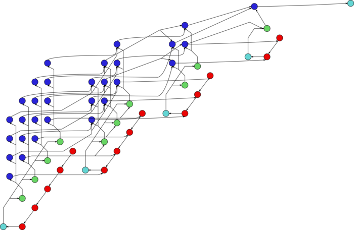
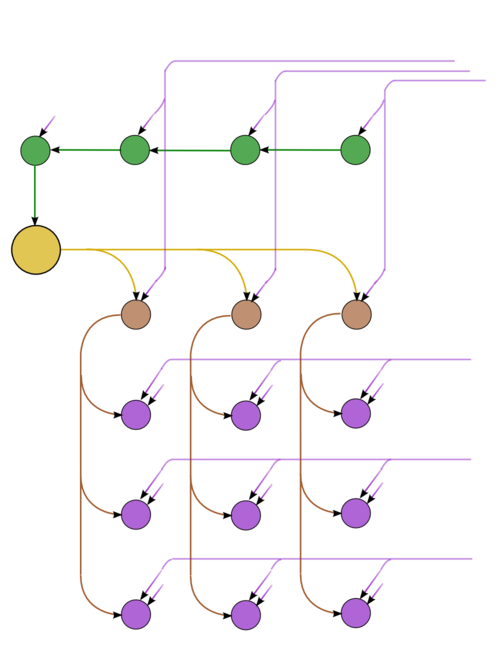
The graph consists of the information graphs of its basic parts. The first part (Gaussian elimination with column pivoting) has the most complex graph. Figure 1 shows the simplified graph of this part, post factum the choice of pivots. The operations of finding the maxima in the columns and saving the corresponding positions are given in green. The inversion of the current pivot, multiplications in the current column, and operations of the type [math]a b + c[/math] in the other columns are depicted in yellow, brown, and purple, respectively. Figure 2 shows the graph of a layer (one step of the method). The notation is the same as in the full graph. Dotted lines denote data communication from the pivot row.

Figure 1. Simplified graph of Gaussian elimination with column pivoting

Figure 2. Graph of one step of Gaussian elimination

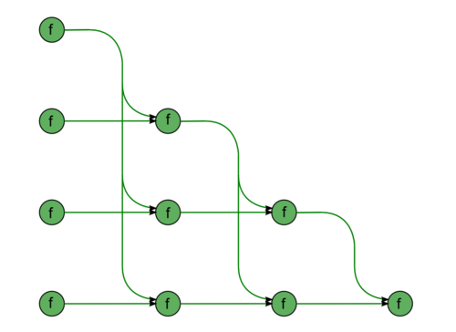
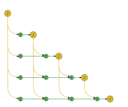
The second part consists of almost identical fragments. The first fragment describes the forward substitution, namely, the solution of the SLAE with a lower triangular matrix [math]L \vec{y} = \vec{b}[/math] (Fig.3). The diagonal entries of this matrix are ones; consequently, this fragment contains no divisions. All the green nodes correspond to the operations of the type [math]a b + c[/math]. The second fragment describes the back substitution, namely, the solution of the SLAE with an upper triangular matrix [math]U \vec{x} = \vec{y}[/math] (Fig.4). This matrix has no specific features; hence, the associated graph contains division operations, which are shown in yellow.

Figure 3. Graph of solving the SLAE with a lower triangular matrix

Figure 4. Graph of solving the SLAE with an upper triangular matrix

1.8 Parallelization resource of the algorithm

The analysis of parallelization resource of the algorithm shows that Gaussian elimination with column pivoting has the highest, namely, quadratic complexity (exactly because of the pivoting). The other parts of the algorithm have at most linear complexity. Therefore, to optimize calculations, the virtual researcher must optimize Gaussian elimination with column pivoting. Besides, the first fragment of the second part (that is, the solution of the first triangular SLAE) can be attached to the first part and executed almost entirely in the background of the latter. Indeed, both have the same direction of recalculating the data. However, the rest of the second part, despite its similarity to the first fragment, can only be executed on completion the latter. The reason is that these two fragments have opposite directions of recalculating the data.

1.9 Input and output data of the algorithm

Actually, this test has always the same data, which are calculated in the test itself. Consequently, in the strict sense, it has no input data.

The output data, produced by the test, are the norms of the residual, solution, and matrix, the ratios of these norms, and the computational power of the target computer system.

2 Software implementation of the algorithm

2.1 Implementation peculiarities of the serial algorithm

Strictly speaking, the investigator implementing the test for a computer system tests at the same time LINPAC or any other package from which procedures for triangular decomposition and solving a SLAE with the help of this decomposition are called. The web versions of the test can also be used for testing other implementations of the Gauss method. It was already noted above that the triangular decomposition of the original matrix is calculated in-place, and, in the course of forward and back substitution, the solutions are written to the locations of right-hand sides. This causes the necessity to regenerate both the coefficient matrix and the right-hand side for the subsequent calculation of the residual. This organization of the algorithm may well be changed in order to optimize the test.

2.2 Locality of data and computations

2.2.1 Locality of implementation

2.2.1.1 Structure of memory access and a qualitative estimation of locality

Figure 5. Linpack benchmark. Overall memory access profile

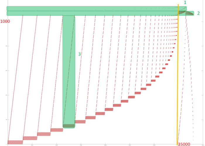
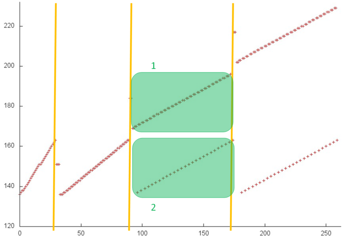
Fig.5 shows the overall memory address profile for the Linpack benchmark. Here, three arrays are used. In Fig.5, the accesses to the first two arrays are distinguished in green (fragments 1 and 2). The other accesses are performed to the entries of the third array, which contains the coefficient matrix of the SLAE. The test consists of two stages, namely, the factorization of the coefficient matrix and the subsequent solution of the SLAE. In figure, the stages are divided by the orange line. One can see that the first stage has an iterative structure, and several matrix entries with smallest indices are dropped from the analysis at each iteration step. One can also notice that the second stage performs two passes with an increasing step over the matrix entries; the first pass is direct, while the second goes in the reverse direction. On the whole, the profile has a fairly complex structure, and a more detailed analysis is needed to understand its locality properties.

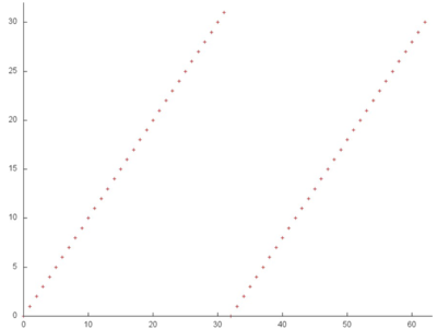
Fragment 1 is shown separately in Fig.6. The fragment is very small compared to the overall profile, but, with this proximity, it is easily seen that this fragment consists of two serial searches of all the array entries. Such a search is characterized by high spatial locality and rather low temporal locality because only two accesses to each entry are performed.

Figure 6. Fragment 1 (access profile for the first array)

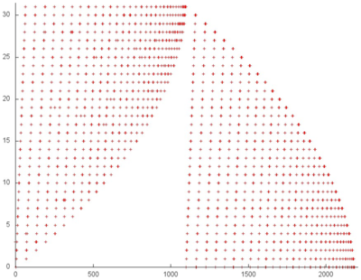
Now, we discuss fragment 2, which is shown in Fig.7. This profile consists of two similar stages; both are sets of iterations. At each iteration step, a serial search is performed, and one array entry is dropped from the analysis. This is the entry with the minimum index, at the first stage, and the entry with the maximum index, at the second stage.

Both the spatial and temporal localities of this profile are very high because the accesses are almost always made to nearby entries; moreover, the entries are fairly easy accessed repeatedly. However, note that this fragment consists of only about 2000 elements, which is considerably less than the overall number of accesses in the program. Consequently, the most of accesses (and, probably, the main impact) are due to the last array.

Figure 7. Fragment 2 (access profile for the second array)

Figure 8 shows fragment 3, selected from fig.5. This fragment depicts one iteration of the loop within which this array is accessed. It is easily seen from the figure that the iteration consists of two parts corresponding to two inner loops. The number of accesses at each iteration of both inner loops is about the same. However, at the next iteration, the first inner loop searches through the next portion of array entries, whereas the second searches through the same entries.

Figure 8. Fragment 3 (access profile for the third array, one iteration)

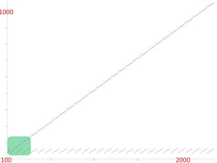
It remains to clarify the structure of memory accesses at the iterations of these two cycles. Consider in more detail the portion of fragment 3, which is shown in green in fig.8 (see fig.9).

Figure 9. Small portion of fragment 3, one iteration

One can see that the first two stages differ from the others because they execute certain initial operations. Then inner loops begin similar iterations; both perform serial searches of entries (see parts 1 and 2 shown in green). The basic difference is that two memory accesses per entry are done within the first loop.

The accesses to this array are characterized by a high spatial locality. Moreover, the second loop always uses the same entries, which also results in a rather high temporal locality. Thus, within one iteration (Fig.4), the locality of accesses is high. If accesses to the same entries are made at different iterations (and the number of accesses per iteration is not very large), then locality improves even further.

2.2.1.2 Quantitative estimation of locality

Основной фрагмент реализации, на основе которого были получены количественные оценки, приведен здесь (оригинал исходного кода взят отсюда). Условия запуска описаны здесь.

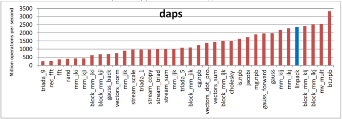
Первая оценка выполняется на основе характеристики daps, которая оценивает число выполненных обращений (чтений и записей) в память в секунду. Данная характеристика является аналогом оценки flops применительно к работе с памятью и является в большей степени оценкой производительности взаимодействия с памятью, чем оценкой локальности. Однако она служит хорошим источником информации, в том числе для сравнения с результатами по следующей характеристике cvg.

На рис.10 приведены значения daps для реализаций распространенных алгоритмов, отсортированные по возрастанию (чем больше daps, тем в общем случае выше производительность). Можно увидеть, что данный показатель у теста Linpack один из самых высоких, что говорит об эффективном взаимодействии с памятью.

Рисунок 10. Сравнение значений оценки daps

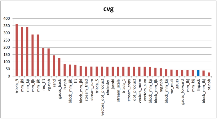
Вторая характеристика – cvg – предназначена для получения более машинно-независимой оценки локальности. Она определяет, насколько часто в программе необходимо подтягивать данные в кэш-память. Соответственно, чем меньше значение cvg, тем реже это нужно делать, тем лучше локальность.

На рис.11 приведены значения cvg для того же набора реализаций, отсортированные по убыванию (чем меньше cvg, тем в общем случае выше локальность). Можно увидеть, что, согласно данной оценке, локальность обращений в память теста Linpack очень высока, что соответствует полученным ранее оценкам и выводам.

Рисунок 11. Сравнение значений оценки cvg

2.4 Scalability of the algorithm and its implementations

2.4.2 Scalability of of the algorithm implementation

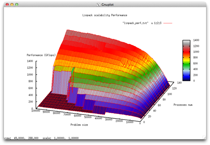
Проведём исследование масштабируемости реализации HPL теста Linpack согласно методике. Исследование проводилось на суперкомпьютере "Ломоносов" Суперкомпьютерного комплекса Московского университета.

Набор и границы значений изменяемых параметров запуска реализации алгоритма:

• число процессоров [8 : 128] с шагом 8;
• размер матрицы [1000 : 100000] c шагом 1000.

В результате проведённых экспериментов был получен следующий диапазон эффективности реализации алгоритма:

• минимальная эффективность реализации 0.039%;
• максимальная эффективность реализации 86,7%.

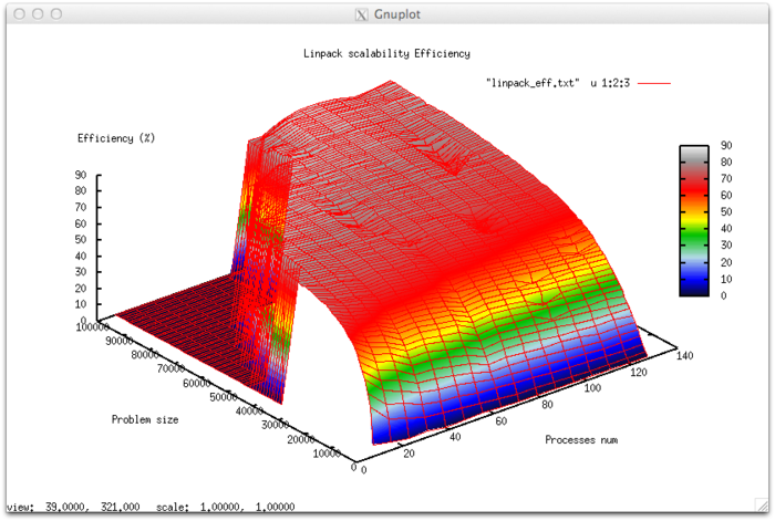
На следующих рисунках приведены графики производительности и эффективности теста HPL в зависимости от изменяемых параметров запуска.

Рисунок 12. Тест HPL. Изменение производительности в зависимости от числа процессоров и размера матрицы.

Рисунок 13. Тест HPL. Изменение производительности в зависимости от числа процессоров и размера матрицы.

Построим оценки масштабируемости теста Linpack:

• По числу процессов: -0.061256. При увеличении числа процессов эффективность на рассмотренной области изменений параметров запуска уменьшается, однако в целом уменьшение не очень быстрое. Малая интенсивность изменения объясняется высокой общей эффективностью работы при больших размерах задачи, однако при росте числа процессов эффективность равномерно уменьшается. Это объясняется также тем, что с ростом вычислительной сложности падение эффективности становится не таким быстрым. Уменьшение эффективности на рассмотренной области работы параллельной программы объясняется быстрым ростом накладных расходов на организацию параллельного выполнения. С ростом вычислительной сложности задачи эффективность снижается так же быстро, но при больших значениях числа процессов. Это подтверждает предположение о том, что накладные расходы начинают сильно превалировать над вычислениями.
• По размеру задачи: 0.010134. При увеличении размера задачи эффективность возрастает. Эффективность возрастает тем быстрее, чем большее число процессов используется для выполнения. Это подтверждает предположение о том, что размер задачи сильно влияет на эффективность выполнения приложения. Оценка показывает, что с ростом размера задачи эффективность на рассмотренной области значений параметров запуска сильно увеличивается. Также, учитывая разницу максимальной и минимальной эффективности почти в 80%, можно сделать вывод, что рост эффективности при увеличении размера задачи наблюдается на большей части рассмотренной области значений.
• По двум направлениям: 0.0000284 При рассмотрении увеличения как вычислительной сложности, так и числа процессов на всей рассмотренной области значений эффективность увеличивается, однако скорость увеличения эффективности не очень большая.

Исследованная реализация теста