Cooley–Tukey Fast Fourier Transform, radix-2 case
Primary authors of this description: A.V.Frolov, Vad.V.Voevodin (Section 2.2)
Contents
- 1 Properties and structure of the algorithm
- 1.1 General description of the algorithm
- 1.2 Mathematical description of the algorithm
- 1.3 Computational kernel of the algorithm
- 1.4 Macro structure of the algorithm
- 1.5 Implementation scheme of the serial algorithm
- 1.6 Serial complexity of the algorithm
- 1.7 Information graph
- 1.8 Parallelization resource of the algorithm
- 1.9 Input and output data of the algorithm
- 1.10 Properties of the algorithm
- 2 Software implementation of the algorithm
- 2.1 Implementation peculiarities of the serial algorithm
- 2.2 Locality of data and computations
- 2.3 Possible methods and considerations for parallel implementation of the algorithm
- 2.4 Scalability of the algorithm and its implementations
- 2.5 Dynamic characteristics and efficiency of the algorithm implementation
- 2.6 Conclusions for different classes of computer architecture
- 2.7 Existing implementations of the algorithm
- 3 References
1 Properties and structure of the algorithm
1.1 General description of the algorithm
Simple Cooley-Tukey algorithm is a variant of Fast Fourier Transform intended for complex vectors of power-of-two size and avoiding special techniques used for sizes equal to power of 4, power of 8, etc.[1] The algorithm repeatedly applies the Fast Fourier Transform and reduces the entire process to a sequence of Fourier transforms of size 2 and multiplications by the so-called twiddle factors. It is slower than Cooley-Tukey algorithms that express a power-of-two size as a power of 4, power of 8, etc. and then use special features of these cases. Nevertheless, this algorithm is widespread for the reason that its program implementation is the simplest of all FFT implementations.
1.2 Mathematical description of the algorithm
Input data: complex vector to be transformed [math]a[/math] (with components [math]a_{i}[/math]).
Output data: complex vector [math]b[/math] (with components [math]b_{i}[/math]), the result of the transform
The size (dimension) of the vectors is [math]n[/math]; moreover, [math]n = 2^l[/math]
1.2.1 Recursive description
The input vector is first written as a sequence of rows, each row containing only two components. Then each row undergoes the Fourier transform of size two. The resulting elements are multiplied by the twiddle factors [math]exp (2 \pi i(m-1)(j-1)/n)[/math] ([math]m[/math] is the row index, and [math]j[/math] is the column index). Finally, each column is processed by the FFT of size [math]n/2[/math]. For the first column, the twiddle factors are equal to 1; hence, no actual multiplication is performed. For the second column, the multiplication by the twiddle factors is combined with the Fourier transform of size two. This combination, called a butterfly by the FFT experts, is the basic operation of the simple Cooley-Tukey algorithm. The butterfly consists in adding two complex numbers and calculating their difference with the subsequent multiplication by another complex number. On the whole, there are [math]n/2[/math] butterflies at each step, while the number of steps is [math]l-1[/math]. Only sums and differences are calculated at the last step [math]l[/math].
1.2.2 Trigonometric functions
Although the calculations described above use the twiddle factors [math]exp (2 \pi i(m-1)(j-1)/n)[/math], it is unreasonable to calculate them while executing the Cooley-Tukey algorithm. Otherwise, the calculations of sines and cosines would constitute the lion's share of all calculations in the algorithm. Usually (and similarly to the other versions of FFT), the twiddle factors are pre-calculated and stored in a separate array. We assume here that the algorithm is executed in exactly this form.
1.3 Computational kernel of the algorithm
The computational kernel of the algorithm is compiled of butterflies. Each butterfly consists in adding two complex numbers and calculating their difference with the subsequent multiplication by another complex number. There are on the whole [math](1/2) n log_{2} n [/math] butterflies. No multiplications are performed in [math]n/2[/math] butterflies.
1.4 Macro structure of the algorithm
The macro structure of the algorithm can best of all be described in a recursive manner, namely, as [math]n/2[/math] Fourier transforms of size two, the multiplication of [math]n/2[/math] pairs of complex numbers, and two FFTs of size [math]n/2[/math].
1.5 Implementation scheme of the serial algorithm
Under the nonrecursive organization scheme, the execution of a butterfly is preceded by partitioning the components into [math]n/2[/math] pairs (there are on the whole [math]log_{2} n [/math] butterflies). At each step, the difference of indices of the elements in a pair is doubled. This difference is 1 at the first step and [math]n/2[/math] at the last step. The result of addition is written into the component with a lesser index, while the result of subtraction and subsequent multiplication is written into the component with a larger index.
1.6 Serial complexity of the algorithm
If the serial complexity is determined by considering only the principal terms of the number of operations, then the simple Cooley-Tukey algorithm requires [math]n log_{2} n[/math] complex additions and [math](1/2) n log_{2} n [/math] complex multiplications. Thus, the simple Cooley-Tukey algorithm can be qualified as a linear logarithmic complexity algorithm.
1.7 Information graph
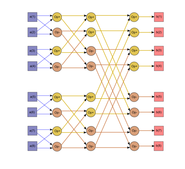
It is evident from the figure that this graph is not linear either in the size or in formulas for its edges. The size of the graph is linear logarithmic, while the edge formulas contain exponentials. At the i-th step, each butterfly involves two components whose indices in their binary representation differ only in the (i-1)-th bit.
1.8 Parallelization resource of the algorithm
If only the principal terms of the number of operations are considered, then the simple Cooley-Tukey algorithm has a critical path formed of [math]log_{2} n [/math] complex additions/subtractions and [math]log_{2} n [/math] complex multiplications. Thus, in terms of parallel complexity, the simple Cooley-Tukey algorithm can be placed into the logarithmic class. In terms of the parallel form width, the complexity of the algorithm is "linear.
1.9 Input and output data of the algorithm
Input data: vector [math]a[/math] (with components [math]a_{i}[/math]).
Size of the input data: [math]n[/math] .
Output data : vector [math]b[/math] (with components [math]b_{i}[/math]).
Size of the output data: [math]n[/math].
1.10 Properties of the algorithm
It is clear that, in the case of unlimited resources, the ratio of the serial to parallel complexity is linear.
The computational power of the algorithm, understood as the ratio of the number of operations to the total size of the input and output data, is logarithmic.
The algorithm is completely determined.
Note that the simple Cooley-Tukey algorithm is not optimal even for vectors of power-of-two size. However, we do not consider any other FFT algorithms here.
2 Software implementation of the algorithm
2.1 Implementation peculiarities of the serial algorithm
In its simplest form, the algorithm can be written in Fortran so that the input and output arrays are the same (the X array is used in this example):
        subroutine STEP2(x,y,pov)
        complex x, y, pov, u, v
        u = x + y
        v = (x-y)*pov
        x = u
        y = v
        return
        end
        subroutine FFT2(X, POV, N, N2, L)
C
C L = Log2N
C N2 = N/2
C
        complex X(0:N-1), POV(0:N2-1)
        DO I = 0, L-1
            DO J = 0, N2/2**I-1
            DO K = 0, 2**I-1
                call STEP2(X(2*J*2**I+K)), X(2*J*2**I+2**I+K), POV(J*2**I-1))
            END DO
            END DO
         END DO
         return
         end
We assume that first-step pivot multipliers (they are also used in subsequent steps) have been pre-computed in advance and are stored in a POV array (with its zero element containing 1). Unfortunately, most implementations of the simple Cooley-Tukey algorithm compute the pivot multipliers simultaneously with “butterfly” computations, which substantially reduces performance.
2.2 Locality of data and computations
2.2.1 Locality of implementation
2.2.1.1 Structure of memory access and a qualitative estimation of locality
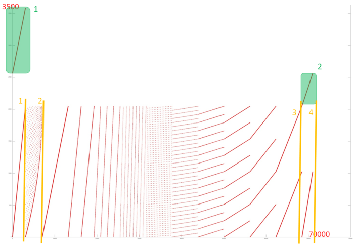
Fig.2 shows the memory call profile for a non-recursive implementation of the Fast Fourier Transformation. As we can see from the source code, the program contains three data arrays. Two of these are highlighted in green in Fig.2, the rest of the profile represents array 3.
Fragments 1 and 2 are formed by calls to input and output arrays, respectively. According to the figure, the fragments look like sequential searches. Analysis of the source code confirms this: in both cases, all elements of the array are searched in a cycle. Such profiles have high spatial locality but low temporal locality, as no element is addressed twice.
The last fragment is much more interesting. It can be broken into four steps, which are highlighted in orange in Fig.2. The first step corresponds in time to Fragment 1, and its profile also looks like a sequential search. The source code confirms that calls within step 1 are related to a ‘data’ array being filled with zeros or values read from the dIn array in Fragment 1:
for( i = 0; i < nn; i++ ) {
data [ i ] = 0;
data[ i * 2 + 1 ] = dIn[ i ];
}
Clearly, calls in step 1 also form a sequential search. Step 4 has a similar structure, but each call from Fragment 1 corresponds to 4 sequential calls in step 4.
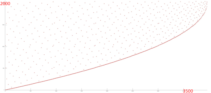
Let’s look at step 2 in more detail (Fig.3). You can see that at the beginning of this step the entire array is called; but the closer to the end of this step, the closer to the end of the array data is accessed. It is obvious that some of the data calls (the bottom curve) are located close to each other, while others are widespread look more like random access.
The source code where memory locations are called at this Step looks as follows:
while( i < n ) {
if( j > i ) {
tempr = data[ i ]; data[ i ] = data[ j ]; data[ j ] = tempr;
tempr = data[ i + 1 ]; data[ i + 1 ] = data[ j + 1 ];
data[ j + 1 ] = tempr;
}
m = n >> 1;
while( ( m >= 2 ) && ( j > m ) ) {
j = j - m;
m = m >> 1;
}
j = j + m;
i = i + 2;
}
You can see that there are indeed two independent indices of memory calls – based on variables i and j; all calls based on i form the curve at the bottom of Fig.3, while j is the variable responsible for all other memory access operations, scattered throughout the array.
It should be noted that calls based on j are not random, but follow a certain law for choosing the next element. However, from a qualitative assessment perspective, these fragments are similar.
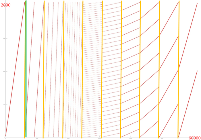
Thus, step 2 consists of two fragments based on two different indices. The first has high spatial locality (a sequential search of array elements) and low temporal locality (each element is only accessed twice). The second has low spatial locality (elements are spread out, except the end of the step) and low temporal locality (each element is accessed only twice). Now let’s move on to the longest step 3, presented individually in Fig.4. Based on the picture, the fragment clearly consists of several iterations: the first iteration consists of a single pass through array elements at some interval; the second iteration consists of two passes with the same interval (bigger than in the first iteration); the third – four passes, etc., until the number of passes per iteration starts falling. The iterations are divided by the orange lines in Fig.4.
It is clear that passes within each iteration have a similar structure; we can also assume that the step is doubled when moving to another iteration, which is confirmed by studying the source code. It can also be seen that each iteration consists of a relatively stable number of calls (the parts highlighted in orange lines are the same size).
The first iteration looks like a sequential search of the array elements and, as such, it has high spatial and temporal locality. As the step increases, spatial locality is reduced, but there is no clarity on what happens to temporal locality – this depends on whether the next pass goes through the same elements. Source code analysis shows that each pass goes over its own elements, so the temporal locality remains low. However, it should be noted that the same elements are used within each iteration, which boosts temporal locality in general.
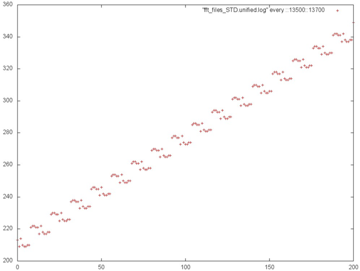
A more detailed study of each pass (see Fig.5, which represents a zoomed-in view of the green area in Fig.4) reveals that its structure is more complex than a simple search through array elements with a certain step: in this case there is a series of calls close to one another, and then a shift by a certain interval. This results in some improvement in both spatial and temporal locality.
2.2.1.2 Quantitative estimation of locality
The key implementation fragment which was used to obtain the quantitative assessment is presented here (Kernel function). Launch conditions are described here.
The first estimate is based on daps, which assesses the number of memory access operations (reads and writes) per second. Similar to flops, this tool is used to evaluate memory access performance, rather than locality. But it is still a good source of information, particularly in combination with the next estimate – cvg.
Fig.6 shows the daps values for implementations of common algorithms sorted in ascending order (larger daps values generally indicate higher performance). You can see that this tool shows low performance, similar to a random access algorithm (rand).
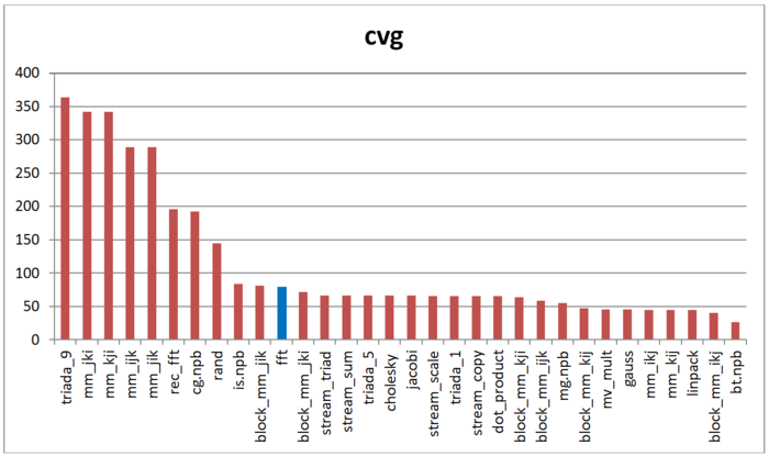
The second tool – cvg – is intended to obtain a more machine-independent locality assessment. It determines how often a program needs to pull data to cache memory. Respectively, the smaller cvg value, the less frequently data needs to be called to cache, and the better the locality.
Fig.7 shows the cvg values for the same set of implementations, sorted in descending order (a lower cvg generally means higher locality). You can see that according to this assessment, this implementation of FFT demonstrates marginally better locality compared to random access or the recursive version, unlike the daps tool that showed almost the same results for these programs. Currently it is unclear what causes this difference. However, it should be noted that the cvg locality assessment is still near the bottom part of the table.
2.3 Possible methods and considerations for parallel implementation of the algorithm
2.4 Scalability of the algorithm and its implementations
2.4.1 Scalability of the algorithm
2.4.2 Scalability of of the algorithm implementation
2.5 Dynamic characteristics and efficiency of the algorithm implementation
2.6 Conclusions for different classes of computer architecture
Of all communication networks, a simple Cooley-Tukey algorithm graph is best reflected on a hypercube type network. The popularity of FFT as a method to address various tasks has therefore popularized the idea of computational systems with a hypercube-type network at the early development stage of various parallel computing systems. Currently, however, these computing systems are not commonly used for physical reasons making a large-dimension hypercube hard to implement in practice. As can be seen from the graph, if it is split into parts by straight lines parallel to the step axis, at the first step there will be no exchange of information between the different parts. But starting at some point, these will grow to an amount comparable to the number of arithmetic operations. This, however, can be avoided by reordering all data in the middle of the algorithm. In the graph, this corresponds to changing the splitting procedure. When these recommendations are followed, the algorithm can be implemented more efficiently than it is at present, and including the use of cluster architecture and other architectures that split a process into independent branches.
2.7 Existing implementations of the algorithm
Simple Cooley-Tukey Fast Fourier Transform algorithm for the powers of two is very common among beginners using FFT, and can easily be found online using search engines. As a result, these implementations do to use the efficiency improvement techniques described above – for sequential or parallel architecture. The reason is that the simple Cooley-Tukey Fast Fourier Transform algorithm for the powers of two is not as good as other Cooley-Tukey algorithms using, for example, the specifics of even powers of two for better efficiency. Therefore most researchers who need faster FFT programs do not try to improve the efficiency of this algorithm, but choose another instead. We recommend that our readers do the same.
3 References
- ↑ Voevodin V.V., Kuznetsov Yu.A. Matrices and computations, Moscow: Nauka, 1984.
