Difference between revisions of "Bellman-Ford algorithm"
| [quality revision] | [quality revision] |
| (52 intermediate revisions by one other user not shown) | |||
| Line 1: | Line 1: | ||
{{algorithm | {{algorithm | ||
| − | | name = | + | | name = Bellman-Ford algorithm |
| serial_complexity = <math>O(|V||E|)</math> | | serial_complexity = <math>O(|V||E|)</math> | ||
| pf_height = <math>N/A, max O(|V|) </math> | | pf_height = <math>N/A, max O(|V|) </math> | ||
| Line 12: | Line 12: | ||
=== General description of the algorithm === | === General description of the algorithm === | ||
| − | ''' | + | The '''Bellman-Ford algorithm'''<ref>Bellman, Richard. “On a Routing Problem.” Quarterly of Applied Mathematics 16 (1958): 87–90.</ref><ref>Ford, L R. Network Flow Theory. Rand.org, RAND Corporation, 1958.</ref><ref>Moore, Edward F. “The Shortest Path Through a Maze,” International Symposium on the Theory of Switching, 285–92, 1959.</ref> was designed for [[Поиск кратчайшего пути от одной вершины (SSSP)|finding the shortest paths between nodes in a graph]]. For a given weighted digraph, the algorithm finds the shortest paths between a singled-out source node and the other nodes of the graph. The Bellman-Ford algorithm scales worse than other algorithms for solving this problem (the complexity is <math>O(|V||E|)</math> against <math>O(|E| + |V|\ln(|V|))</math> for [[Алгоритм Дейкстры|Dijkstra's algorithm]]). However, its distinguishing feature is the applicability to graphs with arbitrary (including negative) weights. |
=== Mathematical description of the algorithm === | === Mathematical description of the algorithm === | ||
| − | + | Let <math>G = (V, E)</math> be a given graph with arc weights <math>f(e)</math> | |
| + | f(e) and the single-out source node <math>u</math>. Denote by <math>d(v)</math> the shortest distance between the source node <math>u</math> and the node <math>v</math>. | ||
| − | + | The Bellman-Ford algorithm finds the value <math>d(v)</math> as the unique solution to the equation | |
:<math> | :<math> | ||
d(v) = \min \{ d(w) + f(e) \mid e = (w, v) \in E \}, \quad \forall v \ne u, | d(v) = \min \{ d(w) + f(e) \mid e = (w, v) \in E \}, \quad \forall v \ne u, | ||
</math> | </math> | ||
| − | + | with the initial condition <math>d(u) = 0</math>. | |
=== Computational kernel of the algorithm === | === Computational kernel of the algorithm === | ||
| − | + | The algorithm is based on the principle of arc relaxation: if <math>e = (w, v) \in E</math> and <math>d(v) > d(w) + f(e)</math>, then the assignment <math>d(v) \leftarrow d(w) + f(e)</math> is performed. | |
=== Macro structure of the algorithm === | === Macro structure of the algorithm === | ||
| − | + | The algorithm successively refines the values of the function <math>d(v)</math>. | |
| − | * | + | * At the very start, the assignment <math>d(u) = 0</math>, <math>d(v) = \infty</math>, <math>\forall v \ne u</math> is performed. |
| − | * | + | * Then <math>|V|-1</math> iteration steps are executed. At each step, all the arcs of the graph undergo the relaxation. |
| − | + | The structure of the algorithm can be described as follows: | |
| − | 1. | + | 1. Initialization: all the nodes are assigned the expected distance <math>t(v)=\infty</math>. The only exception is the source node for which <math>t(u)=0</math> . |
| − | 2. | + | 2. Relaxation of the set of arcs <math>E</math>: |
| − | + | (a) For each arc <math>e=(v,z) \in E</math>, the new expected distance is calculated: <math>t^' (z)=t(v)+ w(e)</math>. | |
| − | + | (b) If <math>t^' (z)< t(z)</math>, then the assignment <math>t(z) := t' (z)</math> (relaxation of the arc <math>e</math>) is performed. | |
| − | 3. | + | 3. The algorithm continues to work as long as at least one arc undergoes relaxation. |
| − | + | Suppose that the relaxation of some arcs was still performed at the <math>|V|</math>-th iteration step. Then the graph contains a cycle of negative length. An arc <math>e=(v,z)</math> lying on such cycle can be found by testing the condition <math>t(v)+w(e)<d(z)</math> (this condition can be verified for all the arcs in linear time). | |
=== Implementation scheme of the serial algorithm === | === Implementation scheme of the serial algorithm === | ||
| − | + | The serial algorithm is implemented by the following pseudo-code: | |
| − | ''' | + | '''Input data''': |
| − | + | graph with nodes ''V'' and arcs ''E'' with weights ''f''(''e''); | |
| − | + | source node ''u''. | |
| − | ''' | + | '''Output data''': distances ''d''(''v'') from the source node ''u'' to each node ''v'' ∈ ''V''. |
'''for each''' ''v'' ∈ ''V'' '''do''' ''d''(''v'') := ∞ | '''for each''' ''v'' ∈ ''V'' '''do''' ''d''(''v'') := ∞ | ||
| Line 67: | Line 68: | ||
=== Serial complexity of the algorithm === | === Serial complexity of the algorithm === | ||
| − | + | The algorithm performs <math>|V|-1</math> iteration steps; at each step, <math>|E|</math> arcs are relaxed. Thus, the total work is <math>O(|V||E|)</math> operations. | |
| − | + | The constant in the complexity estimate can be reduced by using the following two conventional techniques: | |
| − | # | + | # Algorithm terminates if no successful relaxation occurred at the current iteration step. |
| − | # | + | |
| + | # At the current step, not all the arcs are inspected but only the arcs outgoing from nodes that were involved in successful relaxations at the preceding step. (At the first step, only the arcs outgoing from the source node are examined.) | ||
=== Information graph === | === Information graph === | ||
| − | + | The information graph of the Bellman-Ford algorithm is shown in figure 1. It demonstrates the levels of parallelism in this algorithm. | |
| − | [[file:APSP.png|thumb|center|700px| | + | [[file:APSP.png|thumb|center|700px|Figure 1. Information graph of the generalized Bellman-Ford algorithm.]] |
| − | + | The lower level of parallelism refers to operations executed within each horizontal plane. The set of all planes represents the upper level of parallelism (because operations in different planes can be carried out concurrently). | |
| − | + | The lower level of parallelism in the algorithm graph corresponds to levels [2] and [3], which represent the operations of initialization of the distance array ([2]) and updating of this array based on the data in arcs array ([3]). Operation [4] refers to the test whether any changes occurred at the current iteration and the loop termination if no changes were done. | |
| − | + | As already said, the upper level of parallelism consists in the parallel calculation of distances for different source nodes. In the figure, it is illustrated by the set of distinct planes. | |
=== Parallelization resource of the algorithm === | === Parallelization resource of the algorithm === | ||
| − | + | The Bellman-Ford algorithm has a considerable parallelization resource. First, the search for shortest paths can be independently performed for all the nodes (parallel vertical planes in figure 1). Second, the search for shortest paths beginning in a fixed node <math>u</math> can also be made in parallel: the initialization of the original paths ([2]) requires <math>|V|</math> parallel operations, and the relaxation of all arcs costs <math>O(|E|)</math> parallel operations. | |
| − | + | Thus, if <math>O(|E|)</math> processors are available, then the algorithm terminates after at most <math>|V|</math> steps. Actually, a smaller number of steps are usually required, namely, <math>O(r)</math> steps. (This number is the maximum length of the shortest paths outgoing from the chosen source node <math>u</math>). | |
| − | + | It follows that the width of the parallel form of the Bellman-Ford algorithm is <math>O(|E|)</math>, while its height is <math>O(r) | r < |V|</math>. | |
| − | [[ | + | The [[algorithm of Δ-stepping]] can be regarded as a parallel version of the Bellman-Ford algorithm. |
=== Input and output data of the algorithm === | === Input and output data of the algorithm === | ||
| − | ''' | + | '''Input data''': weighted graph <math>(V, E, W)</math> (<math>|V|</math> nodes <math>v_i</math> and <math>|E|</math> arcs <math>e_j = (v^{(1)}_{j}, v^{(2)}_{j})</math> with weights <math>f_j</math>), source node <math>u</math>. |
| + | |||
| + | '''Size of input data''': <math>O(|V| + |E|)</math>. | ||
| − | ''' | + | '''Output data''' (possible variants): |
| − | + | # for each node <math>v</math> of the original graph, the last arc <math>e^*_v = (w, v)</math> lying on the shortest path from <math>u</math> to <math>v</math> or the corresponding node <math>w</math>; | |
| − | # | + | # for each node <math>v</math> of the original graph, the summarized weight <math>f^*(v)</math> of the shortest path from <math>u</math> to <math>v</math>. |
| − | # | ||
| − | ''' | + | '''Size of output data''': <math>O(|V|)</math>. |
=== Properties of the algorithm === | === Properties of the algorithm === | ||
| − | + | The Bellman-Ford algorithm is able to identify cycles of negative length in a graph. An arc <math>e = (v, w)</math> lies on such a cycle if the shortest distances <math>d(v) </math> calculated by the algorithm satisfy the condition | |
:<math> | :<math> | ||
d(v) + f(e) < d(w), | d(v) + f(e) < d(w), | ||
</math> | </math> | ||
| − | + | where <math>f(e)</math> is the weight of the arc <math>e</math>. This condition can be verified for all the arcs of the graph in time <math>O(|E|)</math>. | |
== Software implementation of the algorithm == | == Software implementation of the algorithm == | ||
| Line 124: | Line 127: | ||
===== Structure of memory access and a qualitative estimation of locality ===== | ===== Structure of memory access and a qualitative estimation of locality ===== | ||
| − | [[file:bellman_ford_1.png|thumb|center|700px| | + | [[file:bellman_ford_1.png|thumb|center|700px|Figure 2. Implementation of the Bellman-Ford algorithm. Overall memory access profile]] |
| − | + | Fig.2 shows the memory access profile for an implementation of the Bellman-Ford algorithm. The first thing that should be noted is that the number of memory accesses is much greater than the number of involved data. This says that the data are often used repeatedly, which usually implies high temporal locality. Furthermore, it is evident that the memory accesses have an explicit regular structure; one can also see repeated iterations in the work of the algorithm. Practically all the accesses form fragments similar to a successive search. The upper part of the figure, where the structure is more complicated, is an exception. | |
| − | + | In order to better understand the structure of the overall profile, let us consider more closely its individual areas. Figure 3 shows fragment 1 (selected in fig.2); here, one can see the first 500 memory accesses (note that different slopes of two successive searches are caused by different ratios of sides in the corresponding areas). This figure shows that parts 1 and 2 (selected in yellow) are practically identical successive searches. They only differ in that the accesses in part 1 are performed twice as often compared to part 2; for this reason, the former is represented by a greater number of points. As is known, such profiles are characterized by high spatial and low temporal locality. | |
| − | [[file:bellman_ford_2.png|thumb|center|700px| | + | [[file:bellman_ford_2.png|thumb|center|700px|Figure 3. Memory access profile, fragment 1]] |
| − | + | Now, we consider the more interesting fragment 2 of fig.2 (see fig.4). In the lower area of this profile, one can again see a confirmation of the regularity of accesses. However, its upper area is clearly structured in a more complex way, although the regularity is seen here as well. In particular, the same repeated iterations are present here; in them, one can distinguish long sequences of accesses to the same data. An example of such a behavior, which is optimal in terms of locality, is set out in yellow. | |
| − | [[file:bellman_ford_3.png|thumb|center|700px| | + | [[file:bellman_ford_3.png|thumb|center|700px|Figure 4. Memory access profile, fragment 2]] |
| − | + | In order to understand the structure of memory accesses in the upper area, let us examine this area even more closely. Consider the visualization of the small portion of fragment 2 shown in green in fig.4. In this case, the closer examination (see fig.5) does not make the picture more clear: one can see an irregular structure within an iteration, but the nature of this irregularity is fairly difficult to describe. However, such a description is not required here. Indeed, one can notice that only 15 elements are located along the vertical, whereas the number of accesses to these elements is much greater. Such a profile has a very high locality (both spatial and temporal) regardless of the structure of accesses. | |
| − | [[file:bellman_ford_4.png|thumb|center|700px| | + | [[file:bellman_ford_4.png|thumb|center|700px|Figure 5. A small portion of fragment 2]] |
| − | + | The majority of accesses are performed exactly to fragment 2. Consequently, one can state that the overall profile also has a high spatial and temporal locality. | |
===== Quantitative estimation of locality ===== | ===== Quantitative estimation of locality ===== | ||
| − | + | Our estimate is based on daps, which assesses the number of memory accesses (reads and writes) per second. Similarly to flops, daps is used to evaluate memory access performance rather than locality. Yet, it is a good source of information, particularly for comparison with the results provided by the estimate cvg. | |
| − | + | Fig.6 shows daps values for implementations of popular algorithms, sorted in ascending order (the higher the daps, the better the performance in general). One can see that the memory access performance of this implementation is fairly good. In particular, its daps value is comparable with that for the Linpack benchmark. The latter is known for its high efficiency of memory interaction. | |
| − | [[file:bellman_ford_daps.png|thumb|center|700px| | + | [[file:bellman_ford_daps.png|thumb|center|700px|Figure 6. Comparison of daps values]] |
=== Possible methods and considerations for parallel implementation of the algorithm === | === Possible methods and considerations for parallel implementation of the algorithm === | ||
| − | + | A program implementing the algorithm for finding shortest paths consists of two parts. One part is responsible for the general coordination of computations, as well as parallel computations on a multi-core CPU. The other, GPU part is only responsible for computations on a graphic accelerator. | |
=== Scalability of the algorithm and its implementations === | === Scalability of the algorithm and its implementations === | ||
==== Scalability of the algorithm ==== | ==== Scalability of the algorithm ==== | ||
| − | + | The Bellman-Ford algorithm has a considerable scalability potential because each arc is processed independently of the others, and each computational process can be assigned its own portion of graph arcs. The bottleneck is the access to the distance array shared by all the processes. The algorithm permits to relax requirements to the synchronization of the data in this array between the processes (a process may not immediately see the new value of a distance written by some other process). This possibly can be achieved by performing a greater number of global iterations. | |
| − | ==== Scalability | + | ==== Scalability of the algorithm implementation ==== |
| − | + | Let us study scalability for the parallel implementation of the Bellman-Ford algorithm in accordance with [[Scalability methodology|Scalability methodology]]. This study was conducted using the Lomonosov-2 supercomputer of the [http://parallel.ru/cluster Moscow University Supercomputing Center]. | |
| − | + | Variable parameters for the [[Глоссарий#|start-up]] of the algorithm implementation and the limits of parameter variations: | |
| − | * | + | * number of processors [1 : 28] with the step 1; |
| − | * | + | * graph size [2^20 : 2^27]. |
| − | + | We carry out a separate analysis of the strong scaling-out of the Bellman-Ford algorithm . | |
| − | + | The performance is defined as TEPS (an abbreviation for Traversed Edges Per Second), that is, the number of graph arcs processed by the algorithm in a second. Using this characteristic, one can compare the performance for graphs of different sizes and estimate how the performance gets worse when the graph size increases. | |
| − | [[file:Сильная_масштабируемость_вширь_алгоритма_Беллмана-Форда.png|thumb|center|700px| | + | [[file:Сильная_масштабируемость_вширь_алгоритма_Беллмана-Форда.png|thumb|center|700px|Figure 7. Parallel implementation of the Bellman-Ford algorithm: scalability of different implementations of the algorithm: performance as a function of the graph size]] |
=== Dynamic characteristics and efficiency of the algorithm implementation === | === Dynamic characteristics and efficiency of the algorithm implementation === | ||
| − | + | The experiments were conducted with the Bellman-Ford algorithm implemented for CPU. All the results were obtained with the «Lomonosov-2» supercomputer. We used Intel Xeon E5-2697v3 processors. The problem was solved for a large graph (of size 2^27) on a single node. Only one iteration was performed. The figures below illustrate the efficiency of this implementation. | |
| − | |||
| − | |||
| − | + | [[file:Bellman-Ford cpu.png|thumb|center|700px|Figure 8. Graph of CPU loading while executing the Bellman-Ford algorithm]] | |
| − | + | The graph of CPU loading shows that the processor is idle almost all the time: the average level of loading is about 5 percent. This is a fairly inefficient result even for programs started with the use of only one core. | |
| − | + | [[file:Bellman-Ford LoadAvg.png|thumb|center|700px|Figure 9. Graph of the number of processes expecting the beginning of the calculation stage (Loadavg) while executing the Bellman-Ford algorithm]]The graph of the number of processes expecting the beginning of the calculation stage (Loadavg) shows that the value of this parameter in the course of the program execution is the constant 1. This indicates that the hardware resources are all the time loaded by at most one process. Such a small number points to a not very reasonable use of resources. | |
| − | [[file:Bellman-Ford L1.png|thumb|center|700px| | + | [[file:Bellman-Ford L1.png|thumb|center|700px|Figure 10. Graph of L1 cache misses per second while executing the Bellman-Ford algorithm]] |
| − | + | The graph of L1 cache misses shows that the number of misses is very large. It is on the level of 140 millions per second, which is a very high value indicating a potential cause of inefficiency. | |
| − | [[file:Bellman-Ford L2.png|thumb|center|700px| | + | [[file:Bellman-Ford L2.png|thumb|center|700px|Figure 11. Graph of L2 cache misses per second while executing the Bellman-Ford algorithm]] |
| − | + | The graph of L2 cache misses shows that the number of such misses is also very large. It is on the level of 140 millions per second, which indicates an extremely inefficient memory interaction. | |
| − | [[file:Bellman-Ford-L3.png|thumb|center|700px| | + | [[file:Bellman-Ford-L3.png|thumb|center|700px|Figure 12. Graph of L3 cache misses per second while executing the Bellman-Ford algorithm]] |
| − | + | The graph of L3 cache misses shows that the number of these misses is again large; it is about 30 millions per second. This indicates that the problem fits very badly into cache memory, and the program is compelled to work all the time with RAM, which is explained by the very large size of the input graph. | |
| − | [[file:Bellman-Ford Inf Data.png|thumb|center|700px| | + | [[file:Bellman-Ford Inf Data.png|thumb|center|700px|Figure 13. Graph of the data rate through Infiniband network (in bytes per second) while executing the Bellman-Ford algorithm]] |
| − | + | The graph of the data rate through Infiniband network shows a fairly high intensity of using this network at the first stage. This is explained by the program logic, which assumes the reading of the graph from a disc file. On Lomonosov-2, communications with this disc are performed through a dedicated Infiniband network. | |
| − | [[file:Bellman-Ford Inf Pckts.png|thumb|center|700px| | + | [[file:Bellman-Ford Inf Pckts.png|thumb|center|700px|Figure 14. Graph of the data rate through Infiniband network (in packets per second) while executing the Bellman-Ford algorithm]] |
| − | + | The graph of the data rate measured in packets per second demonstrates a similar picture of very high intensity at the first stage of executing the problem. Later on, the network is almost not used. | |
| − | + | On the whole, the data of system monitoring make it possible to conclude that the program worked with a stable intensity. However, it used the memory very inefficiently due to the extremely large size of the graph. | |
=== Conclusions for different classes of computer architecture === | === Conclusions for different classes of computer architecture === | ||
=== Existing implementations of the algorithm === | === Existing implementations of the algorithm === | ||
| − | * C++: [http://www.boost.org/libs/graph/doc/ Boost Graph Library] ( | + | * C++: [http://www.boost.org/libs/graph/doc/ Boost Graph Library] (function <code>[http://www.boost.org/libs/graph/doc/bellman_ford_shortest.html bellman_ford_shortest]</code>). |
| − | * Python: [https://networkx.github.io NetworkX] ( | + | * Python: [https://networkx.github.io NetworkX] (function <code>[http://networkx.github.io/documentation/networkx-1.9.1/reference/generated/networkx.algorithms.shortest_paths.weighted.bellman_ford.html bellman_ford]</code>). |
| − | * Java: [http://jgrapht.org JGraphT] ( | + | * Java: [http://jgrapht.org JGraphT] (class <code>[http://jgrapht.org/javadoc/org/jgrapht/alg/BellmanFordShortestPath.html BellmanFordShortestPath]</code>). |
== References == | == References == | ||
Revision as of 14:53, 5 February 2018
| Bellman-Ford algorithm | |
| Sequential algorithm | |
| Serial complexity | [math]O(|V||E|)[/math] |
| Input data | [math]O(|V| + |E|)[/math] |
| Output data | [math]O(|V|^2)[/math] |
| Parallel algorithm | |
| Parallel form height | [math]N/A, max O(|V|) [/math] |
| Parallel form width | [math]O(|E|)[/math] |
Contents
- 1 Properties and structure of the algorithm
- 1.1 General description of the algorithm
- 1.2 Mathematical description of the algorithm
- 1.3 Computational kernel of the algorithm
- 1.4 Macro structure of the algorithm
- 1.5 Implementation scheme of the serial algorithm
- 1.6 Serial complexity of the algorithm
- 1.7 Information graph
- 1.8 Parallelization resource of the algorithm
- 1.9 Input and output data of the algorithm
- 1.10 Properties of the algorithm
- 2 Software implementation of the algorithm
- 2.1 Implementation peculiarities of the serial algorithm
- 2.2 Locality of data and computations
- 2.3 Possible methods and considerations for parallel implementation of the algorithm
- 2.4 Scalability of the algorithm and its implementations
- 2.5 Dynamic characteristics and efficiency of the algorithm implementation
- 2.6 Conclusions for different classes of computer architecture
- 2.7 Existing implementations of the algorithm
- 3 References
1 Properties and structure of the algorithm
1.1 General description of the algorithm
The Bellman-Ford algorithm[1][2][3] was designed for finding the shortest paths between nodes in a graph. For a given weighted digraph, the algorithm finds the shortest paths between a singled-out source node and the other nodes of the graph. The Bellman-Ford algorithm scales worse than other algorithms for solving this problem (the complexity is [math]O(|V||E|)[/math] against [math]O(|E| + |V|\ln(|V|))[/math] for Dijkstra's algorithm). However, its distinguishing feature is the applicability to graphs with arbitrary (including negative) weights.
1.2 Mathematical description of the algorithm
Let [math]G = (V, E)[/math] be a given graph with arc weights [math]f(e)[/math] f(e) and the single-out source node [math]u[/math]. Denote by [math]d(v)[/math] the shortest distance between the source node [math]u[/math] and the node [math]v[/math].
The Bellman-Ford algorithm finds the value [math]d(v)[/math] as the unique solution to the equation
- [math] d(v) = \min \{ d(w) + f(e) \mid e = (w, v) \in E \}, \quad \forall v \ne u, [/math]
with the initial condition [math]d(u) = 0[/math].
1.3 Computational kernel of the algorithm
The algorithm is based on the principle of arc relaxation: if [math]e = (w, v) \in E[/math] and [math]d(v) \gt d(w) + f(e)[/math], then the assignment [math]d(v) \leftarrow d(w) + f(e)[/math] is performed.
1.4 Macro structure of the algorithm
The algorithm successively refines the values of the function [math]d(v)[/math].
- At the very start, the assignment [math]d(u) = 0[/math], [math]d(v) = \infty[/math], [math]\forall v \ne u[/math] is performed.
- Then [math]|V|-1[/math] iteration steps are executed. At each step, all the arcs of the graph undergo the relaxation.
The structure of the algorithm can be described as follows:
1. Initialization: all the nodes are assigned the expected distance [math]t(v)=\infty[/math]. The only exception is the source node for which [math]t(u)=0[/math] .
2. Relaxation of the set of arcs [math]E[/math]:
(a) For each arc [math]e=(v,z) \in E[/math], the new expected distance is calculated: [math]t^' (z)=t(v)+ w(e)[/math].
(b) If [math]t^' (z)\lt t(z)[/math], then the assignment [math]t(z) := t' (z)[/math] (relaxation of the arc [math]e[/math]) is performed.
3. The algorithm continues to work as long as at least one arc undergoes relaxation.
Suppose that the relaxation of some arcs was still performed at the [math]|V|[/math]-th iteration step. Then the graph contains a cycle of negative length. An arc [math]e=(v,z)[/math] lying on such cycle can be found by testing the condition [math]t(v)+w(e)\lt d(z)[/math] (this condition can be verified for all the arcs in linear time).
1.5 Implementation scheme of the serial algorithm
The serial algorithm is implemented by the following pseudo-code:
Input data:
  graph with nodes V and arcs E with weights f(e);
  source node u.
Output data: distances d(v) from the source node u to each node  v ∈ V.

for each v ∈ V do d(v) := ∞
d(u) = 0

for i from 1 to |V| - 1:
    for each e = (w, v) ∈ E:
        if d(v) > d(w) + f(e):
            d(v) := d(w) + f(e)
1.6 Serial complexity of the algorithm
The algorithm performs [math]|V|-1[/math] iteration steps; at each step, [math]|E|[/math] arcs are relaxed. Thus, the total work is [math]O(|V||E|)[/math] operations.
The constant in the complexity estimate can be reduced by using the following two conventional techniques:
- Algorithm terminates if no successful relaxation occurred at the current iteration step.
- At the current step, not all the arcs are inspected but only the arcs outgoing from nodes that were involved in successful relaxations at the preceding step. (At the first step, only the arcs outgoing from the source node are examined.)
1.7 Information graph
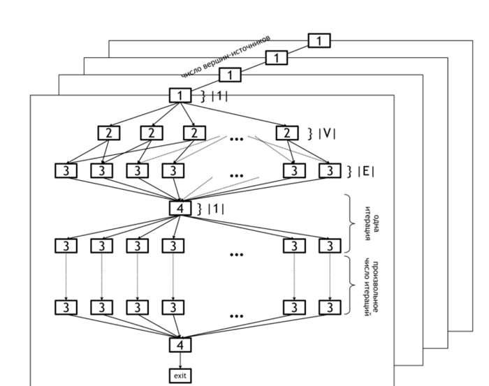
The information graph of the Bellman-Ford algorithm is shown in figure 1. It demonstrates the levels of parallelism in this algorithm.
The lower level of parallelism refers to operations executed within each horizontal plane. The set of all planes represents the upper level of parallelism (because operations in different planes can be carried out concurrently).
The lower level of parallelism in the algorithm graph corresponds to levels [2] and [3], which represent the operations of initialization of the distance array ([2]) and updating of this array based on the data in arcs array ([3]). Operation [4] refers to the test whether any changes occurred at the current iteration and the loop termination if no changes were done.
As already said, the upper level of parallelism consists in the parallel calculation of distances for different source nodes. In the figure, it is illustrated by the set of distinct planes.
1.8 Parallelization resource of the algorithm
The Bellman-Ford algorithm has a considerable parallelization resource. First, the search for shortest paths can be independently performed for all the nodes (parallel vertical planes in figure 1). Second, the search for shortest paths beginning in a fixed node [math]u[/math] can also be made in parallel: the initialization of the original paths ([2]) requires [math]|V|[/math] parallel operations, and the relaxation of all arcs costs [math]O(|E|)[/math] parallel operations.
Thus, if [math]O(|E|)[/math] processors are available, then the algorithm terminates after at most [math]|V|[/math] steps. Actually, a smaller number of steps are usually required, namely, [math]O(r)[/math] steps. (This number is the maximum length of the shortest paths outgoing from the chosen source node [math]u[/math]).
It follows that the width of the parallel form of the Bellman-Ford algorithm is [math]O(|E|)[/math], while its height is [math]O(r) | r \lt |V|[/math].
The algorithm of Δ-stepping can be regarded as a parallel version of the Bellman-Ford algorithm.
1.9 Input and output data of the algorithm
Input data: weighted graph [math](V, E, W)[/math] ([math]|V|[/math] nodes [math]v_i[/math] and [math]|E|[/math] arcs [math]e_j = (v^{(1)}_{j}, v^{(2)}_{j})[/math] with weights [math]f_j[/math]), source node [math]u[/math].
Size of input data: [math]O(|V| + |E|)[/math].
Output data (possible variants):
- for each node [math]v[/math] of the original graph, the last arc [math]e^*_v = (w, v)[/math] lying on the shortest path from [math]u[/math] to [math]v[/math] or the corresponding node [math]w[/math];
- for each node [math]v[/math] of the original graph, the summarized weight [math]f^*(v)[/math] of the shortest path from [math]u[/math] to [math]v[/math].
Size of output data: [math]O(|V|)[/math].
1.10 Properties of the algorithm
The Bellman-Ford algorithm is able to identify cycles of negative length in a graph. An arc [math]e = (v, w)[/math] lies on such a cycle if the shortest distances [math]d(v) [/math] calculated by the algorithm satisfy the condition
- [math] d(v) + f(e) \lt d(w), [/math]
where [math]f(e)[/math] is the weight of the arc [math]e[/math]. This condition can be verified for all the arcs of the graph in time [math]O(|E|)[/math].
2 Software implementation of the algorithm
2.1 Implementation peculiarities of the serial algorithm
2.2 Locality of data and computations
2.2.1 Locality of implementation
2.2.1.1 Structure of memory access and a qualitative estimation of locality
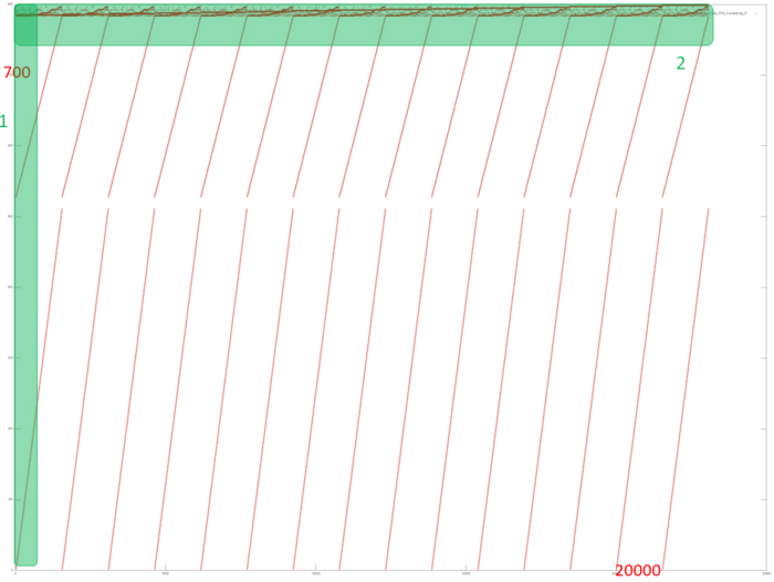
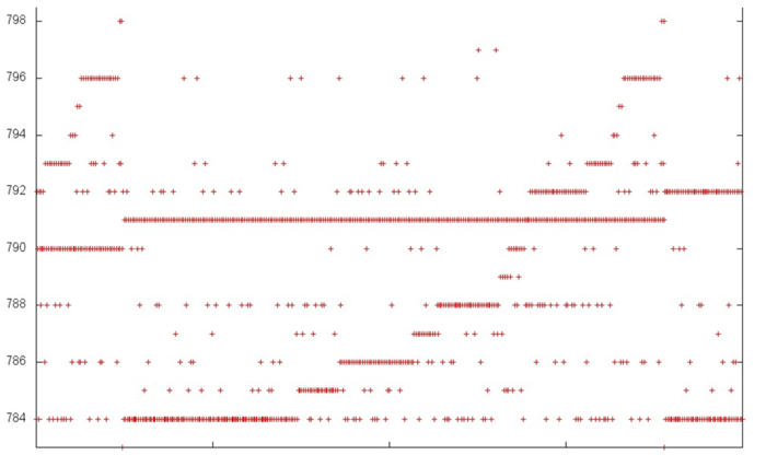
Fig.2 shows the memory access profile for an implementation of the Bellman-Ford algorithm. The first thing that should be noted is that the number of memory accesses is much greater than the number of involved data. This says that the data are often used repeatedly, which usually implies high temporal locality. Furthermore, it is evident that the memory accesses have an explicit regular structure; one can also see repeated iterations in the work of the algorithm. Practically all the accesses form fragments similar to a successive search. The upper part of the figure, where the structure is more complicated, is an exception.
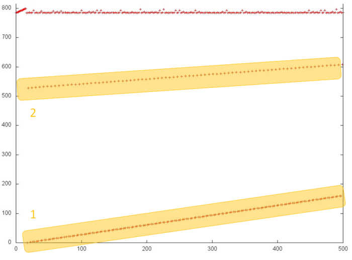
In order to better understand the structure of the overall profile, let us consider more closely its individual areas. Figure 3 shows fragment 1 (selected in fig.2); here, one can see the first 500 memory accesses (note that different slopes of two successive searches are caused by different ratios of sides in the corresponding areas). This figure shows that parts 1 and 2 (selected in yellow) are practically identical successive searches. They only differ in that the accesses in part 1 are performed twice as often compared to part 2; for this reason, the former is represented by a greater number of points. As is known, such profiles are characterized by high spatial and low temporal locality.
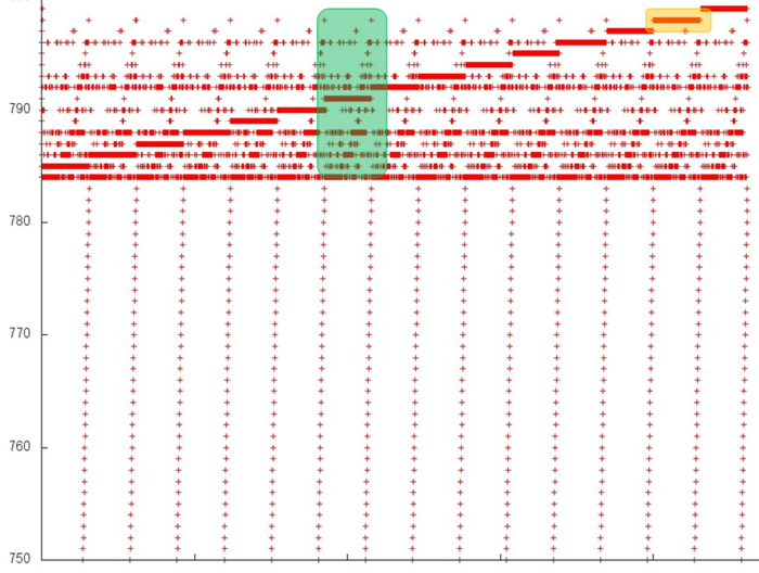
Now, we consider the more interesting fragment 2 of fig.2 (see fig.4). In the lower area of this profile, one can again see a confirmation of the regularity of accesses. However, its upper area is clearly structured in a more complex way, although the regularity is seen here as well. In particular, the same repeated iterations are present here; in them, one can distinguish long sequences of accesses to the same data. An example of such a behavior, which is optimal in terms of locality, is set out in yellow.
In order to understand the structure of memory accesses in the upper area, let us examine this area even more closely. Consider the visualization of the small portion of fragment 2 shown in green in fig.4. In this case, the closer examination (see fig.5) does not make the picture more clear: one can see an irregular structure within an iteration, but the nature of this irregularity is fairly difficult to describe. However, such a description is not required here. Indeed, one can notice that only 15 elements are located along the vertical, whereas the number of accesses to these elements is much greater. Such a profile has a very high locality (both spatial and temporal) regardless of the structure of accesses.
The majority of accesses are performed exactly to fragment 2. Consequently, one can state that the overall profile also has a high spatial and temporal locality.
2.2.1.2 Quantitative estimation of locality
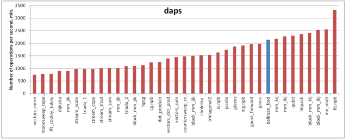
Our estimate is based on daps, which assesses the number of memory accesses (reads and writes) per second. Similarly to flops, daps is used to evaluate memory access performance rather than locality. Yet, it is a good source of information, particularly for comparison with the results provided by the estimate cvg.
Fig.6 shows daps values for implementations of popular algorithms, sorted in ascending order (the higher the daps, the better the performance in general). One can see that the memory access performance of this implementation is fairly good. In particular, its daps value is comparable with that for the Linpack benchmark. The latter is known for its high efficiency of memory interaction.
2.3 Possible methods and considerations for parallel implementation of the algorithm
A program implementing the algorithm for finding shortest paths consists of two parts. One part is responsible for the general coordination of computations, as well as parallel computations on a multi-core CPU. The other, GPU part is only responsible for computations on a graphic accelerator.
2.4 Scalability of the algorithm and its implementations
2.4.1 Scalability of the algorithm
The Bellman-Ford algorithm has a considerable scalability potential because each arc is processed independently of the others, and each computational process can be assigned its own portion of graph arcs. The bottleneck is the access to the distance array shared by all the processes. The algorithm permits to relax requirements to the synchronization of the data in this array between the processes (a process may not immediately see the new value of a distance written by some other process). This possibly can be achieved by performing a greater number of global iterations.
2.4.2 Scalability of the algorithm implementation
Let us study scalability for the parallel implementation of the Bellman-Ford algorithm in accordance with Scalability methodology. This study was conducted using the Lomonosov-2 supercomputer of the Moscow University Supercomputing Center.
Variable parameters for the start-up of the algorithm implementation and the limits of parameter variations:
- number of processors [1 : 28] with the step 1;
- graph size [2^20 : 2^27].
We carry out a separate analysis of the strong scaling-out of the Bellman-Ford algorithm .
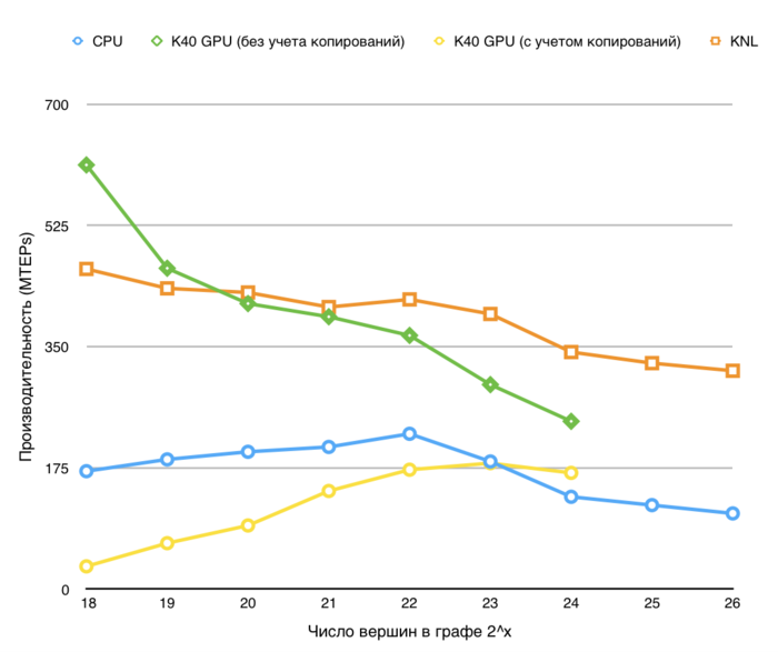
The performance is defined as TEPS (an abbreviation for Traversed Edges Per Second), that is, the number of graph arcs processed by the algorithm in a second. Using this characteristic, one can compare the performance for graphs of different sizes and estimate how the performance gets worse when the graph size increases.
2.5 Dynamic characteristics and efficiency of the algorithm implementation
The experiments were conducted with the Bellman-Ford algorithm implemented for CPU. All the results were obtained with the «Lomonosov-2» supercomputer. We used Intel Xeon E5-2697v3 processors. The problem was solved for a large graph (of size 2^27) on a single node. Only one iteration was performed. The figures below illustrate the efficiency of this implementation.
The graph of CPU loading shows that the processor is idle almost all the time: the average level of loading is about 5 percent. This is a fairly inefficient result even for programs started with the use of only one core.
The graph of the number of processes expecting the beginning of the calculation stage (Loadavg) shows that the value of this parameter in the course of the program execution is the constant 1. This indicates that the hardware resources are all the time loaded by at most one process. Such a small number points to a not very reasonable use of resources.
The graph of L1 cache misses shows that the number of misses is very large. It is on the level of 140 millions per second, which is a very high value indicating a potential cause of inefficiency.
The graph of L2 cache misses shows that the number of such misses is also very large. It is on the level of 140 millions per second, which indicates an extremely inefficient memory interaction.
The graph of L3 cache misses shows that the number of these misses is again large; it is about 30 millions per second. This indicates that the problem fits very badly into cache memory, and the program is compelled to work all the time with RAM, which is explained by the very large size of the input graph.
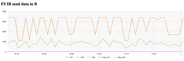
The graph of the data rate through Infiniband network shows a fairly high intensity of using this network at the first stage. This is explained by the program logic, which assumes the reading of the graph from a disc file. On Lomonosov-2, communications with this disc are performed through a dedicated Infiniband network.
The graph of the data rate measured in packets per second demonstrates a similar picture of very high intensity at the first stage of executing the problem. Later on, the network is almost not used.
On the whole, the data of system monitoring make it possible to conclude that the program worked with a stable intensity. However, it used the memory very inefficiently due to the extremely large size of the graph.
2.6 Conclusions for different classes of computer architecture
2.7 Existing implementations of the algorithm
- C++: Boost Graph Library (function
bellman_ford_shortest). - Python: NetworkX (function
bellman_ford). - Java: JGraphT (class
BellmanFordShortestPath).
