Gaussian elimination, compact scheme for tridiagonal matrices, serial variant

Gaussian elimination, compact scheme for tridiagonal matrices, serial variant
Sequential algorithm
Serial complexity	[math]3n-3[/math]
Input data	[math]3n-2[/math]
Output data	[math]3n-2[/math]
Parallel algorithm
Parallel form height	[math]3n-3[/math]
Parallel form width	[math]1[/math]

Main authors: Alexey Frolov

1 Properties and structure of the algorithm

1.1 General description of the algorithm

Сompact scheme for Gaussian elimination, as applied to tri-diagonal matrices, calculates the [math]LU[/math] decomposition of a tri-diagonal matrix

[math] A = \begin{bmatrix} a_{11} & a_{12} & 0 & \cdots & \cdots & 0 \\ a_{21} & a_{22} & a_{23}& \cdots & \cdots & 0 \\ 0 & a_{32} & a_{33} & \cdots & \cdots & 0 \\ \vdots & \vdots & \ddots & \ddots & \ddots & 0 \\ 0 & \cdots & \cdots & a_{n-1 n-2} & a_{n-1 n-1} & a_{n-1 n} \\ 0 & \cdots & \cdots & 0 & a_{n n-1} & a_{n n} \\ \end{bmatrix} [/math]

into the product of bi-diagonal matrices

[math] L = \begin{bmatrix} 1 & 0 & 0 & \cdots & \cdots & 0 \\ l_{21} & 1 & 0 & \cdots & \cdots & 0 \\ 0 & l_{32} & 1 & \cdots & \cdots & 0 \\ \vdots & \vdots & \ddots & \ddots & \ddots & 0 \\ 0 & \cdots & \cdots & l_{n-1 n-2} & 1 & 0 \\ 0 & \cdots & \cdots & 0 & l_{n n-1} & 1 \\ \end{bmatrix} [/math]

and

[math] U = \begin{bmatrix} u_{11} & u_{12} & 0 & \cdots & \cdots & 0 \\ 0 & u_{22} & u_{23}& \cdots & \cdots & 0 \\ 0 & 0 & u_{33} & \cdots & \cdots & 0 \\ \vdots & \vdots & \ddots & \ddots & \ddots & 0 \\ 0 & \cdots & \cdots & 0 & u_{n-1 n-1} & u_{n-1 n} \\ 0 & \cdots & \cdots & 0 & 0 & u_{n n} \\ \end{bmatrix} [/math].

The choice of fixed values for the diagonal entries of [math]L[/math] makes all the nonzero entries in the decomposition uniquely determined (up to round-off errors). The compact scheme provides natural formulas for these entries. The [math]LU[/math] decomposition of a tri-diagonal matrix is a particular case of the general compact scheme for Gaussian elimination. However, the specificity of the tri-diagonal case drastically changes the characteristics of the algorithm compared to the compact scheme for dense matrices.

1.2 Mathematical description of the algorithm

The formulas of the algorithm are as follows:

[math]u_{11} = a_{11} [/math]

[math]u_{i i+1} = a_{i i+1}, \quad i \in [1, n-1] [/math]

[math]l_{i+1 i} = a_{i+1 i} / u_{i i} , \quad i \in [1, n-1] [/math]

[math]u_{ii} = a_{ii} - l_{i i-1} u_{i-1 i}, \quad i \in [2, n] [/math]

1.3 Computational kernel of the algorithm

The above formulas show that the same sequence of three arithmetic operations (division, multiplication, and subtraction) is repeated n-1 times.

1.4 Macro structure of the algorithm

The sequence of three operations (division, multiplication, and subtraction) can be taken as a macro-vertex. In the algorithm, these macro-vertices are performed n-1 times.

1.5 Implementation scheme of the serial algorithm

The scheme takes into account that a number of output data need not be calculated because they are identical to the corresponding data. In particular,

[math]u_{11} = a_{11} [/math]

[math]u_{i i+1} = a_{i i+1}, \quad i \in [1, n-1][/math].

At the start of the process, [math]i = 1[/math]

1. Calculate [math]l_{i+1 i} = a_{i+1 i} / u_{i i}[/math]

Increase [math]i[/math] by 1

2. Calculate [math]u_{ii} = a_{ii} - l_{i i-1} u_{i-1 i}[/math]

If [math]i = n[/math], then exit; otherwise, return to Step 1.

1.6 Serial complexity of the algorithm

The serial variant of the compact scheme of Gaussian elimination, as applied to the decomposition of a tri-diagonal matrix of order n, requires

• [math]n-1[/math] divisions,
• [math]n-1[/math] multiplications,
• [math]n-1[/math] additions (subtractions).

Thus, in terms of serial complexity, the serial variant of the compact scheme of Gaussian elimination, as applied to the decomposition of a tri-diagonal matrix, is qualified as a linear complexity algorithm.

1.7 Information graph

• 

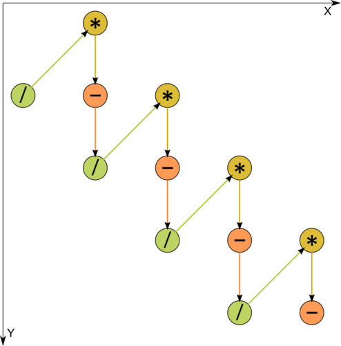
  Figure 1. Graph of the algorithm. The input and output data are not shown. / - division, * - multiplication, - - subtraction.

• 

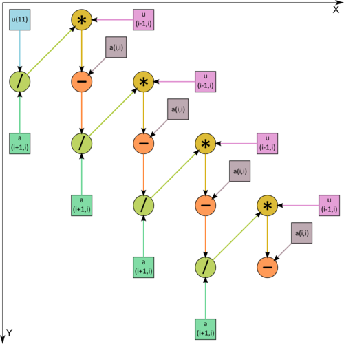
  Figure 2. Graph of the algorithm. The input data are shown. / - division, * - multiplication, - - subtraction.

One can see from Figure 1, where one of the operations is decomposed into two constituents, that the information graph is purely serial.

1.8 Parallelization resource of the algorithm

In order to factorize a tri-diagonal matrix of order n by using the compact scheme of Gaussian elimination, one should perform

• [math]n-1[/math] layers of division,
• [math]n-1[/math] layers of multiplication,
• [math]n-1[/math] layers of addition (subtraction).

Each layer consists of a single operation. Hence, in terms of the parallel form height, the compact scheme of Gaussian elimination for factoring tri-diagonal matrices, in its serial version, is a linear complexity algorithm. The layer width is everywhere equal to 1. Thus, the entire algorithm is an all-over bottleneck.

1.9 Input and output data of the algorithm

Input data: tri-diagonal matrix [math]A[/math] (with entries [math]a_{ij}[/math]).

Size of the input data: [math]3n-2[/math]. Different implementations may store the information differently for economy reasons. For instance, each diagonal of the matrix can be stored by a separate row of the array.

Output data: lower bi-diagonal matrix [math]L[/math] (with entries [math]l_{ij}[/math], where [math]l_{ii}=1[/math]) and upper bi-diagonal matrix [math]U[/math] (with entries [math]u_{ij}[/math]).

Size of the output data is formally [math]3n-2[/math]. However, since [math]n[/math] items in the input and output data are identical, actually only [math]2n-2[/math] items are calculated.

1.10 Properties of the algorithm

It is clear that, in the case of unlimited resources, the ratio of the serial to parallel complexity is one (that is, the algorithm is non-parallelizable).

The computational power of the algorithm, understood as the ratio of the number of operations to the total size of the input and output data, is only a constant (the number of arithmetic operations is the same as the size of the data).

The algorithm is completely determined.

The equivalent perturbation [math]M[/math] of the algorithm does not exceed the perturbation [math]\delta A[/math] that results from inputting the data into memory: [math] ||M||_{E} \leq ||\delta A||_{E} [/math]

2 Software implementation of the algorithm

2.1 Implementation peculiarities of the serial algorithm

In its simplest version, the algorithm can be written in Fortran as follows:

	DO  I = 1, N-1
		A(I+1,I) = A(I+1,I)/A(I,I)
                A(I+1,I+1) = A(I+1,I+1) - A(I+1,I)*A(I,I+1)
	END DO

The decomposition is stored at the place where the original matrix was stored. The indexing is the same as for a dense matrix.

However, much more often, more economical schemes are used for storing tri-diagonal matrices. For instance, assume that the diagonals are numbered from left to right and each diagonal is stored by a separate row of the array. Then the following version is obtained:

	DO  I = 1, N-1
		A(1,I) = A(1,I)/A(2,I)
                A(2,I+1) = A(2,I+1) - A(1,I)*A(3,I)
	END DO

Here, the decomposition also overrides the original data. Элементы A(1,N) и A(3,N) при данном способе хранения не адресуются.

2.2 Locality of data and computations

По приведённым фрагментам программ видно, что степень локальности данных и вычислений очень высока. Особенно это выражено для второго варианта, в котором все данные, как используемые операцией, так и вычисляемые ей, хранятся и используются "рядом". Однако выигрыш от столь высокой локальности, однако, ограничен тем, что каждое перевычисляемое данное используется затем только однажды. Это вызвано простой причиной: количество обрабатываемых алгоритмом данных, как уже описано выше, равно количеству арифметических операций.

2.3 Possible methods and considerations for parallel implementation of the algorithm

Компактная схема метода Гаусса в применении к разложению трёхдиагональной матрицы - это чисто последовательный алгоритм. Его невозможно исполнять параллельно из-за того, что каждая из операций требует в качестве данных результат предыдущей и сама, в свою очередь, отдаёт результат как входное данное для следующей.

Варианты распараллеливания компактной схемы метода Гаусса для трёхдиагональной матрицы используют ассоциативность операций, и, следовательно, представляют собой совсем другие алгоритмы, которые можно изучить на соответствующей странице.

Кроме этого, возможен случай, когда нужны многие разложения разных трёхдиагональных матриц, тогда этот последовательный алгоритм может быть параллельно выполнен для этих матриц на разных узлах вычислительной системы.

2.4 Scalability of the algorithm and its implementations

При чисто последовательном характере алгоритма его ресурсы параллельности полностью отсутствуют: выгоднее все вычисления проводить на одном процессоре.

2.6 Conclusions for different classes of computer architecture

Из-за последовательной структуры более или менее эффективно алгоритм в своём неизменном виде может быть выполнен только на вычислителе классической фон-неймановской архитектуры.