Difference between revisions of "Givens method"
| [unchecked revision] | [checked revision] |
| (47 intermediate revisions by 5 users not shown) | |||
| Line 1: | Line 1: | ||
| + | {{algorithm | ||
| + | | name = Givens (rotation) method for the<br />QR decomposition of a square matrix | ||
| + | | serial_complexity = <math>2 n^3</math> | ||
| + | | input_data = <math>n^2</math> | ||
| + | | output_data = <math>n^2</math> | ||
| + | | pf_height = <math>11n-16</math> | ||
| + | | pf_width = <math>O(n^2)</math> | ||
| + | }} | ||
| + | Primary authors of this description: [[:ru:Участник:Frolov|Alexey Frolov]]. | ||
| + | == Properties and structure of the algorithm == | ||
| − | + | === General description of the algorithm === | |
| + | '''Givens method''' (which is also called '''the rotation method''' in the Russian mathematical literature) is used to represent a matrix in the form <math>A = QR</math>, where <math>Q</math> is a unitary and <math>R</math> is an upper triangular matrix<ref>V.V. Voevodin, Yu.A. Kuznetsov. Matrices and Computations. Moscow, Nauka, 1984 (in Russian).</ref>. The matrix <math>Q</math> is not stored and used in its explicit form but rather as the product of rotations. Each (Givens) rotation can be specified by a pair of indices and a single parameter. | ||
| − | + | {{Template:Rotation matrix}} | |
| − | + | In a conventional implementation of Givens method, this fact makes it possible to avoid using additional arrays by storing the results of decomposition in the array originally occupied by <math>A</math>. Various uses are possible for the <math>QR</math> decomposition of <math>A</math>. It can be used for solving a SLAE (System of Linear Algebraic Equations) <math>Ax = b</math> or as a step in the so-called <math>QR</math> algorithm for finding the eigenvalues of a matrix. | |
| − | + | At each step of Givens method, two rows of the matrix under transformation are rotated. The parameter of this transformation is chosen so as to eliminate one of the entries in the current matrix. First, the entries in the first column are eliminated one after the other, then the same is done for the second column, etc., until the column <math>n-1</math>. The resulting matrix is <math>R</math>. The step of the method is split into two parts: the choice of the rotation parameter and the rotation itself performed over two rows of the current matrix. The entries of these rows located to the left of the pivot column are zero; thus, no modifications are needed there. The entries in the pivot column are rotated simultaneously with the choice of the rotation parameter. Hence, the second part of the step consists in rotating two-dimensional vectors formed of the entries of the rotated rows that are located to the right of the pivot column. In terms of operations, the update of a column is equivalent to multiplying two complex numbers (or to four multiplications, one addition and one subtraction for real numbers); one of these complex numbers is of modulus 1. The choice of the rotation parameter from the two entries of the pivot column is a more complicated procedure, which is explained, in particular, by the necessity of minimizing roundoff errors. The tangent <math>t</math> of half the rotation angle is normally used to store information about the rotation matrix. The cosine <math>c</math> and the sine <math>s</math> of the rotation angle itself are related to <math>t</math> via the basic trigonometry formulas | |
| − | |||
| − | |||
| − | |||
| − | |||
| − | |||
| − | At each step of Givens | ||
<math>c = (1 - t^2)/(1 + t^2), s = 2t/(1 + t^2)</math> | <math>c = (1 - t^2)/(1 + t^2), s = 2t/(1 + t^2)</math> | ||
| − | It is the value <math>t</math> that is usually stored in the corresponding array entry. | + | It is the value <math>t</math> that is usually stored in the corresponding array entry. |
| − | + | === Mathematical description of the algorithm === | |
In order to obtain the <math>QR</math> decomposition of a square matrix <math>A</math>, this matrix is reduced to the upper triangular matrix <math>R</math> (where <math>R</math> means right) by successively multiplying <math>A</math> on the left by the rotations <math>T_{1 2}, T_{1 3}, ..., T_{1 n}, T_{2 3}, T_{2 4}, ..., T_{2 n}, ... , T_{n-2 n}, T_{n-1 n}</math>. | In order to obtain the <math>QR</math> decomposition of a square matrix <math>A</math>, this matrix is reduced to the upper triangular matrix <math>R</math> (where <math>R</math> means right) by successively multiplying <math>A</math> on the left by the rotations <math>T_{1 2}, T_{1 3}, ..., T_{1 n}, T_{2 3}, T_{2 4}, ..., T_{2 n}, ... , T_{n-2 n}, T_{n-1 n}</math>. | ||
| Line 33: | Line 38: | ||
To complete this mathematical description, it remains to specify how the rotation <math>T_{i j}</math> is calculated | To complete this mathematical description, it remains to specify how the rotation <math>T_{i j}</math> is calculated | ||
| − | <ref name="VOLA"> | + | <ref name="VOLA">V.V. Voevodin. Computational Foundations of Linear Algebra. Moscow, Nauka, 1977 (in Russian).</ref> and list the formulas for rotating the current intermediate matrix. |
Let the matrix to be transformed contain the number <math>x</math> in its position <math>(i,i)</math> and the number <math>y</math> in the position <math>(i,j)</math>. Then, to minimize roundoff errors, we first calculate the uniform norm of the vector <math>z = max (|x|,|y|)</math>. | Let the matrix to be transformed contain the number <math>x</math> in its position <math>(i,i)</math> and the number <math>y</math> in the position <math>(i,j)</math>. Then, to minimize roundoff errors, we first calculate the uniform norm of the vector <math>z = max (|x|,|y|)</math>. | ||
| Line 45: | Line 50: | ||
Let the parameters <math>c</math> and <math>s</math> of the rotation <math>T_{i j}</math> have already been obtained. Then the transformation of each column located to the right of the <math>i</math>-th column can be described in a simple way. Let the <math>k</math>-th column have x as its component <math>i</math> and y as its component <math>j</math>. The updated values of these components are <math>cx - sy</math> and <math>sx + cy</math>, respectively. This calculation is equivalent to multiplying the complex number with the real part <math>x</math> and the imaginary part <math>y</math> by the complex number <math>(c,s)</math>. | Let the parameters <math>c</math> and <math>s</math> of the rotation <math>T_{i j}</math> have already been obtained. Then the transformation of each column located to the right of the <math>i</math>-th column can be described in a simple way. Let the <math>k</math>-th column have x as its component <math>i</math> and y as its component <math>j</math>. The updated values of these components are <math>cx - sy</math> and <math>sx + cy</math>, respectively. This calculation is equivalent to multiplying the complex number with the real part <math>x</math> and the imaginary part <math>y</math> by the complex number <math>(c,s)</math>. | ||
| − | + | === Computational kernel of the algorithm === | |
| − | |||
The computational kernel of this algorithm can be thought of as compiled of two types of operation. The first type concerns the calculation of rotation parameters, while the second deals with the rotation itself (which can equivalently be described as the multiplication of two complex numbers with one of the factors having the modulus 1). | The computational kernel of this algorithm can be thought of as compiled of two types of operation. The first type concerns the calculation of rotation parameters, while the second deals with the rotation itself (which can equivalently be described as the multiplication of two complex numbers with one of the factors having the modulus 1). | ||
| − | + | === Macro structure of the algorithm === | |
| − | |||
The operations related to the calculation of rotation parameters can be represented by a triangle on a two-dimensional grid, while the rotation itself can be represented by a pyramid on a three-dimensional grid. | The operations related to the calculation of rotation parameters can be represented by a triangle on a two-dimensional grid, while the rotation itself can be represented by a pyramid on a three-dimensional grid. | ||
| + | === Implementation scheme of the serial algorithm === | ||
| − | + | In a conventional implementation scheme, the algorithm is written as the successive elimination of the subdiagonal entries of a matrix beginning from its first column and ending with the penultimate column (that is, column <math>n-1</math>). When the <math>i</math>-th column is "eliminated", then its components <math>i+1</math> to <math>n</math> are successively eliminated. | |
| − | |||
| − | In a conventional implementation scheme, the algorithm is written as the successive elimination of the subdiagonal entries of a matrix beginning from its first column and ending with the penultimate column (that is, column n-1). When the i-th column is "eliminated", then its components i+1 to n are successively eliminated. | ||
| − | The elimination of the entry (j, i) consists of two steps: (a) calculating the parameters for the rotation | + | The elimination of the entry <math>(j, i)</math> consists of two steps: (a) calculating the parameters for the rotation |
| − | <math>T_{ij}</math> that eliminates the entry (j, i); (b) multiplying the current matrix on the left by the rotation | + | <math>T_{ij}</math> that eliminates the entry <math>(j, i)</math>; (b) multiplying the current matrix on the left by the rotation |
<math>T_{ij}</math>. | <math>T_{ij}</math>. | ||
| − | + | === Serial complexity of the algorithm === | |
| − | |||
The complexity of the serial version of this algorithm is basically determined by the mass rotation operations. If possible sparsity of a matrix is ignored, these operations are responsible (in the principal term) for | The complexity of the serial version of this algorithm is basically determined by the mass rotation operations. If possible sparsity of a matrix is ignored, these operations are responsible (in the principal term) for | ||
<math>n^3/3</math> complex multiplications. In a straightforward complex arithmetic, this is equivalent to <math>4n^3/3</math> real multiplications and <math>2n^3/3</math> real additions/subtractions. | <math>n^3/3</math> complex multiplications. In a straightforward complex arithmetic, this is equivalent to <math>4n^3/3</math> real multiplications and <math>2n^3/3</math> real additions/subtractions. | ||
| − | Thus, in terms of serial complexity, Givens | + | Thus, in terms of serial complexity, Givens method is qualified as a cubic complexity algorithm. |
| − | + | === Information graph === | |
| − | |||
The macrograph of the algorithm is shown in fig. 1, while the graphs of the macrovertices are depicted in the subsequent figures. | The macrograph of the algorithm is shown in fig. 1, while the graphs of the macrovertices are depicted in the subsequent figures. | ||
| − | Figure 1. Graph of the algorithm (the input and output data are not shown). n=4. F1 denotes an operation of calculating rotation parameters, and F2 denotes a rotation of a 2-dimensional vector (which is equivalent to multiplying two complex numbers) | + | [[file:Givens graph.png|thumb|center|600px|Figure 1. Graph of the algorithm (the input and output data are not shown). n=4. F1 denotes an operation of calculating rotation parameters, and F2 denotes a rotation of a 2-dimensional vector (which is equivalent to multiplying two complex numbers)]] |
| − | Choice of a method for calculating rotation parameters in vertices of type F1. | + | <center> |
| − | + | <div class="thumb"> | |
| + | <div class="thumbinner" style="width:{{#expr: 3 * (400 + 35) + 4 * (3 - 1) + 8}}px"> | ||
| + | <gallery widths=400px heights=400px> | ||
| + | File:F1-full.png|Figure 2. Choice of a method for calculating rotation parameters in vertices of type F1 | ||
| + | File:Givens F1!=.png|Figure 3. Calculation of the rotation parameters for various x and y in the vertex V2 | ||
| + | File:Givens F1==.png|Figure 4. Calculation of the rotation parameters in the vertex V0 (the case of zero x and у) | ||
| + | </gallery> | ||
| + | </div> | ||
| + | </div> | ||
| − | Figure | + | <div class="thumb"> |
| − | + | <div class="thumbinner" style="width:{{#expr: 3 * (400 + 35) + 4 * (3 - 1) + 8}}px"> | |
| + | <gallery widths=400px heights=300px> | ||
| + | File:Givens F1=0.png|Figure 5. Calculation of the rotation parameters in the vertex V0 (the case of zero x and у) | ||
| + | File:Povorot-complexmult.png|Figure 6. The inner graph of a vertex of type F2 with its input and output parameters: (u,v) = (c,s)(x,y) | ||
| + | </gallery> | ||
| + | </div> | ||
| + | </div> | ||
| + | </center> | ||
| − | + | <center> | |
| − | + | <tabs> | |
| + | <tab name="n=3"> | ||
| + | {{#widget:Algoviewer | ||
| + | |url=Givens/giv3/Algo_view_givens3.html | ||
| + | |width=1300 | ||
| + | |height=800 | ||
| + | |border=1 | ||
| + | }} | ||
| + | </tab> | ||
| + | <tab name="n=4"> | ||
| + | {{#widget:Algoviewer | ||
| + | |url=Givens/giv4/Algo_view_givens4.html | ||
| + | |width=1300 | ||
| + | |height=800 | ||
| + | |border=1 | ||
| + | }} | ||
| + | </tab> | ||
| + | </tabs> | ||
| + | </center> | ||
| − | + | === Parallelization resource of the algorithm === | |
| − | + | In order to better understand the parallelization resource of Givens' decomposition of a matrix of order <math>n</math>, consider the critical path of its graph. | |
| − | |||
| − | |||
| − | |||
| − | |||
| − | |||
| − | In order to better understand the parallelization resource of Givens' decomposition of a matrix of order n, consider the critical path of its graph. | ||
It is evident from the description of subgraphs that the macrovertex F1 (calculation of the rotation parameters) is much more "weighty" than the rotation vertex F2. Namely, the critical path of a rotation vertex consists of only one multiplication (there are four multiplications, but all of them can be performed in parallel) and one addition/subtraction (there are two operations of this sort, but they also are parallel). On the other hand, in the worst case, a macrovertex for calculating rotation parameters has the critical path consisting of a single square root calculation, two divisions, two multiplications, and two additions/subtractions. | It is evident from the description of subgraphs that the macrovertex F1 (calculation of the rotation parameters) is much more "weighty" than the rotation vertex F2. Namely, the critical path of a rotation vertex consists of only one multiplication (there are four multiplications, but all of them can be performed in parallel) and one addition/subtraction (there are two operations of this sort, but they also are parallel). On the other hand, in the worst case, a macrovertex for calculating rotation parameters has the critical path consisting of a single square root calculation, two divisions, two multiplications, and two additions/subtractions. | ||
| − | According to a rough estimate, the critical path goes through 2n-3 macrovertices of type F1 (calculating rotation parameters) and n-1 rotation macrovertices. Altogether, this yields a critical path passing through 2n-3 square root extractions, 4n-6 divisions, 5n-7 multiplications, and the same number of additions/subtractions. In the macrograph shown in the figure, one of the critical paths consists of the passage through the upper line of F1 vertices (there are n-1 vertices) accompanied by the alternate execution of F2 and F1 (n-2 times) and the final execution of F2. | + | According to a rough estimate, the critical path goes through <math>2n-3</math> macrovertices of type F1 (calculating rotation parameters) and <math>n-1</math> rotation macrovertices. Altogether, this yields a critical path passing through <math>2n-3</math> square root extractions, <math>4n-6</math> divisions, <math>5n-7</math> multiplications, and the same number of additions/subtractions. In the macrograph shown in the figure, one of the critical paths consists of the passage through the upper line of F1 vertices (there are <math>n-1</math> vertices) accompanied by the alternate execution of F2 and F1 (<math>n-2</math> times) and the final execution of F2. |
| − | Thus, unlike in the serial | + | Thus, unlike in the serial version, square root calculations and divisions take a fairly considerable portion of the overall time required for the parallel variant. The presence of isolated square root calculations and divisions in some layers of the parallel form can also create other problems when the algorithm is implemented for a specific architecture. Consider, for instance, an implementation for PLDs. Other operations (multiplications and additions/subtractions) can be pipelined, which also saves resources. On the other hand, isolated square root calculations take resources that are idle most of the time. |
In terms of the parallel form height, the Givens method is qualified as a ''linear complexity'' algorithm. In terms of the parallel form width, its complexity is ''quadratic''. | In terms of the parallel form height, the Givens method is qualified as a ''linear complexity'' algorithm. In terms of the parallel form width, its complexity is ''quadratic''. | ||
| + | === Input and output data of the algorithm === | ||
| − | ''' | + | '''Input data''': dense square matrix <math>A</math> (with entries <math>a_{ij}</math>). |
| − | ''' | + | '''Size of the input data''': <math>n^2</math>. |
| − | ''' | + | '''Output data''': upper triangular matrix <math>R</math> (in the serial version, the nonzero entries <math>r_{ij}</math> are stored in the positions of the original entries <math>a_{ij}</math>), unitary (or orthogonal) matrix <math>Q</math> stored as the product of rotations (in the serial version, the rotation parameters <math>t_{ij}</math> are stored in the positions of the original entries <math>a_{ij}</math>). |
| − | ''' | + | '''Size of the output data''': <math>n^2</math>. |
| − | + | === Properties of the algorithm === | |
| − | |||
| − | |||
| − | |||
It is clearly seen that the ratio of the serial to parallel complexity is ''quadratic'', which is a good incentive for parallelization. | It is clearly seen that the ratio of the serial to parallel complexity is ''quadratic'', which is a good incentive for parallelization. | ||
| Line 126: | Line 151: | ||
Within the framework of the chosen version, the algorithm is completely determined. | Within the framework of the chosen version, the algorithm is completely determined. | ||
| − | The roundoff errors in Givens | + | The roundoff errors in Givens (rotations) method grow ''linearly'', as they also do in Householder (reflections) method. |
| − | |||
| − | + | == Software implementation of the algorithm == | |
| − | + | === Implementation peculiarities of the serial algorithm === | |
| − | In its simplest version, the QR decomposition of a real square matrix by Givens | + | In its simplest version, the QR decomposition of a real square matrix by Givens method can be written in Fortran as follows: |
| + | <source lang="fortran"> | ||
DO I = 1, N-1 | DO I = 1, N-1 | ||
DO J = I+1, N | DO J = I+1, N | ||
| Line 143: | Line 168: | ||
END DO | END DO | ||
END DO | END DO | ||
| + | </source> | ||
Suppose that the translator at hand competently implements operations with complex numbers. Then the rotation subroutine ROT2D can be written as follows: | Suppose that the translator at hand competently implements operations with complex numbers. Then the rotation subroutine ROT2D can be written as follows: | ||
| + | <source lang="fortran"> | ||
SUBROUTINE ROT2D (C, S, X, Y) | SUBROUTINE ROT2D (C, S, X, Y) | ||
COMPLEX Z | COMPLEX Z | ||
| Line 155: | Line 182: | ||
RETURN | RETURN | ||
END | END | ||
| + | </source> | ||
or | or | ||
| + | <source lang="fortran"> | ||
SUBROUTINE ROT2D (C, S, X, Y) | SUBROUTINE ROT2D (C, S, X, Y) | ||
ZZ = C*X - S*Y | ZZ = C*X - S*Y | ||
| Line 162: | Line 191: | ||
RETURN | RETURN | ||
END | END | ||
| + | </source> | ||
(from the viewpoint of the algorithm graph, these subroutines are equivalent). | (from the viewpoint of the algorithm graph, these subroutines are equivalent). | ||
| Line 167: | Line 197: | ||
The subroutine for calculating the rotation parameters can have the following form: | The subroutine for calculating the rotation parameters can have the following form: | ||
| + | <source lang="fortran"> | ||
SUBROUTINE PARAMS (X, Y, C, S) | SUBROUTINE PARAMS (X, Y, C, S) | ||
Z = MAX (ABS(X), ABS(Y)) | Z = MAX (ABS(X), ABS(Y)) | ||
| Line 192: | Line 223: | ||
RETURN | RETURN | ||
END | END | ||
| + | </source> | ||
In the above implementation, the rotation parameter t is written to a vacant location (the entry of the modified matrix with the corresponding indices is known to be zero). This makes it possible to readily reconstruct rotation matrices (if required). | In the above implementation, the rotation parameter t is written to a vacant location (the entry of the modified matrix with the corresponding indices is known to be zero). This makes it possible to readily reconstruct rotation matrices (if required). | ||
| + | === Possible methods and considerations for parallel implementation of the algorithm === | ||
| − | + | On cluster-like supercomputers, a partitioning of an algorithm (with the usage of coordinate generalized schedule of | |
| − | + | the algorithm graph) and its distribution between different nodes (MPI) are fairly possible. At the same time, the inner parallelism in blocks will partially realize multi-core node capabilities (OpenMP) and even core superscalarity. This should be the aim of an implementation judging by the structure of the graph algorithm. | |
| − | |||
| − | + | The structure of the graph makes one think that a good scalability can be attained, although, at the moment, this guess cannot be verified through concrete implementations. The favorable factors are a good (linear) nature of the critical path and a good coordinate structure of generalized schedule, which permits a good block partitioning of the algorithm graph. | |
| − | + | An unexpected result was obtained by a search through the available program packages<ref>A.V. Frolov, A.S. Antonov, Vl.V. Voevodin, A.M. Teplov. Comparison of different methods for solving the same problem on the basis of Algowiki methodology (in Russian) // Submitted to the conference "Parallel computational technologies (PaVT'2016)".</ref>. Most of old (serial) packages contain a subroutine for the QR decomposition via Givens method. By contrast, new packages, intended for parallel execution, perform the QR decomposition solely on the basis of Householder (reflections) method. Meanwhile, parallel properties of the latter are inferior to those of Givens method. We attribute this fact to that Householder method can | |
| + | easily be written in terms of BLAS-procedures, and it does not require loop reordering (except for the case where a partitioning is used; however, in this case, the coordinate rather than skewed loop partitioning is applied). On the other hand, some loop rewriting is needed for the parallel implementation of Givens method because skewed parallelism should be applied to achieve the maximum degree in its parallelization. Thus, we cannot assess the scalability of this algorithm implementations for the reason that no such implementations exist at the moment. | ||
| − | + | === Run results === | |
| + | === Conclusions for different classes of computer architecture === | ||
| − | + | The module for calculating rotation parameters has a complicated logical structure. Therefore, we recommend the reader not to use PLDs as accelerators of universal processors for the reason that a significant part of their equipment will be idle. Certain difficulties are also possible on architectures with universal processors; however, the general structure of the algorithm makes it possible to expect a good performance from such architectures. For instance, on cluster-like supercomputers, a partitioning of the algorithm and its distribution between different nodes are fairly possible. At the same time, the inner parallelism in blocks will partially realize multi-core node capabilities and even core superscalarity. | |
| − | + | == References == | |
| − | + | <references /> | |
| − | |||
| − | + | [[Ru: Метод Гивенса (вращений) QR-разложения квадратной матрицы (вещественный точечный вариант)]] | |
| − | |||
| − | |||
| − | |||
| − | |||
| − | |||
| − | + | [[Category:Finished articles]] | |
| − | |||
| − | |||
Latest revision as of 16:32, 8 July 2022
| Givens (rotation) method for the QR decomposition of a square matrix | |
| Sequential algorithm | |
| Serial complexity | [math]2 n^3[/math] |
| Input data | [math]n^2[/math] |
| Output data | [math]n^2[/math] |
| Parallel algorithm | |
| Parallel form height | [math]11n-16[/math] |
| Parallel form width | [math]O(n^2)[/math] |
Primary authors of this description: Alexey Frolov.
Contents
- 1 Properties and structure of the algorithm
- 1.1 General description of the algorithm
- 1.2 Mathematical description of the algorithm
- 1.3 Computational kernel of the algorithm
- 1.4 Macro structure of the algorithm
- 1.5 Implementation scheme of the serial algorithm
- 1.6 Serial complexity of the algorithm
- 1.7 Information graph
- 1.8 Parallelization resource of the algorithm
- 1.9 Input and output data of the algorithm
- 1.10 Properties of the algorithm
- 2 Software implementation of the algorithm
- 3 References
1 Properties and structure of the algorithm
1.1 General description of the algorithm
Givens method (which is also called the rotation method in the Russian mathematical literature) is used to represent a matrix in the form [math]A = QR[/math], where [math]Q[/math] is a unitary and [math]R[/math] is an upper triangular matrix[1]. The matrix [math]Q[/math] is not stored and used in its explicit form but rather as the product of rotations. Each (Givens) rotation can be specified by a pair of indices and a single parameter.
colomn numbers: [math]\begin{matrix} \ _{i-1}\quad _i\quad _{i+1} & \ & _{j-1}\ \ _j\quad _{j+1}\end{matrix}[/math]
[math]T_{ij} = \begin{bmatrix} 1 & \cdots & 0\quad 0\quad 0 & \cdots & 0\quad 0\quad 0 & \cdots & 0 \\ \vdots & \ddots & \vdots & \vdots & \vdots & \vdots \\ 0 & \cdots & 1\quad 0\quad 0 & \cdots & 0\quad 0\quad 0 & \cdots & 0 \\ 0 & \cdots & 0\quad c\quad 0 & \cdots & 0\ -s\ 0 & \cdots & 0 \\ 0 & \cdots & 0\quad 0\quad 1 & \cdots & 0\quad 0\quad 0 & \cdots & 0 \\ \vdots & \vdots & \vdots & \ddots & \vdots & \vdots & \vdots \\ 0 & \cdots & 0\quad 0\quad 0 & \cdots & 1\quad 0\quad 0 & \cdots & 0 \\ 0 & \cdots & 0\quad s\quad 0 & \cdots & 0\quad c\quad 0 & \cdots & 0 \\ 0 & \cdots & 0\quad 0\quad 0 & \cdots & 0\quad 0\quad 1 & \cdots & 0 \\ \vdots & \vdots & \vdots & \vdots & \vdots & \ddots & \vdots \\ 0 & \cdots & 0\quad 0\quad 0 & \cdots & 0\quad 0\quad 0 & \cdots & 1 \\ \end{bmatrix} [/math]
In a conventional implementation of Givens method, this fact makes it possible to avoid using additional arrays by storing the results of decomposition in the array originally occupied by [math]A[/math]. Various uses are possible for the [math]QR[/math] decomposition of [math]A[/math]. It can be used for solving a SLAE (System of Linear Algebraic Equations) [math]Ax = b[/math] or as a step in the so-called [math]QR[/math] algorithm for finding the eigenvalues of a matrix.
At each step of Givens method, two rows of the matrix under transformation are rotated. The parameter of this transformation is chosen so as to eliminate one of the entries in the current matrix. First, the entries in the first column are eliminated one after the other, then the same is done for the second column, etc., until the column [math]n-1[/math]. The resulting matrix is [math]R[/math]. The step of the method is split into two parts: the choice of the rotation parameter and the rotation itself performed over two rows of the current matrix. The entries of these rows located to the left of the pivot column are zero; thus, no modifications are needed there. The entries in the pivot column are rotated simultaneously with the choice of the rotation parameter. Hence, the second part of the step consists in rotating two-dimensional vectors formed of the entries of the rotated rows that are located to the right of the pivot column. In terms of operations, the update of a column is equivalent to multiplying two complex numbers (or to four multiplications, one addition and one subtraction for real numbers); one of these complex numbers is of modulus 1. The choice of the rotation parameter from the two entries of the pivot column is a more complicated procedure, which is explained, in particular, by the necessity of minimizing roundoff errors. The tangent [math]t[/math] of half the rotation angle is normally used to store information about the rotation matrix. The cosine [math]c[/math] and the sine [math]s[/math] of the rotation angle itself are related to [math]t[/math] via the basic trigonometry formulas
[math]c = (1 - t^2)/(1 + t^2), s = 2t/(1 + t^2)[/math]
It is the value [math]t[/math] that is usually stored in the corresponding array entry.
1.2 Mathematical description of the algorithm
In order to obtain the [math]QR[/math] decomposition of a square matrix [math]A[/math], this matrix is reduced to the upper triangular matrix [math]R[/math] (where [math]R[/math] means right) by successively multiplying [math]A[/math] on the left by the rotations [math]T_{1 2}, T_{1 3}, ..., T_{1 n}, T_{2 3}, T_{2 4}, ..., T_{2 n}, ... , T_{n-2 n}, T_{n-1 n}[/math].
Each [math]T_{i j}[/math] specifies a rotation in the two-dimensional subspace determined by the [math]i[/math]-th and [math]j[/math]-th components of the corresponding column; all the other components are not changed. The rotation is chosen so as to eliminate the entry in the position ([math]i[/math], [math]j[/math]). Zero vectors do not change under rotations and identity transformations; therefore, the subsequent rotations preserve zeros that were earlier obtained to the left and above the entry under elimination.
At the end of the process, we obtain [math]R=T_{n-1 n}T_{n-2 n}T_{n-2 n-1}...T_{1 3}T_{1 2}A[/math].
Since rotations are unitary matrices, we naturally have [math]Q=(T_{n-1 n}T_{n-2 n}T_{n-2 n-1}...T_{1 3}T_{1 2})^* =T_{1 2}^* T_{1 3}^* ...T_{1 n}^* T_{2 3}^* T_{2 4}^* ...T_{2 n}^* ...T_{n-2 n}^* T_{n-1 n}^*[/math] and [math]A=QR[/math].
In the real case, rotations are orthogonal matrices; hence, [math]Q=(T_{n-1 n}T_{n-2 n}T_{n-2 n-1}...T_{1 3}T_{1 2})^T =T_{1 2}^T T_{1 3}^T ...T_{1 n}^T T_{2 3}^T T_{2 4}^T ...T_{2 n}^T ...T_{n-2 n}^T T_{n-1 n}^T[/math].
To complete this mathematical description, it remains to specify how the rotation [math]T_{i j}[/math] is calculated [2] and list the formulas for rotating the current intermediate matrix.
Let the matrix to be transformed contain the number [math]x[/math] in its position [math](i,i)[/math] and the number [math]y[/math] in the position [math](i,j)[/math]. Then, to minimize roundoff errors, we first calculate the uniform norm of the vector [math]z = max (|x|,|y|)[/math].
If the norm is zero, then no rotation is required: [math]t=s=0, c=1[/math].
If [math]z=|x|[/math], then we calculate [math]y_1=y/x[/math] and, next, [math]c = \frac {1}{\sqrt{1+y_1^2}}[/math], [math]s=-c y_1[/math], [math]t=\frac {1-\sqrt{1+y_1^2}}{y_1}[/math]. The updated value of the entry [math](i,i)[/math] is [math]x \sqrt{1+y_1^2}[/math].
If [math]z=|y|[/math], then we calculate [math]x_1=x/y[/math] and, next, [math]t=x_1 - x_1^2 sign(x_1)[/math], [math]s=\frac{sign(x_1)}{\sqrt{1+x_1^2}}[/math], [math]c = s x_1[/math]. The updated value of the entry [math](i,i)[/math] is [math]y \sqrt{1+x_1^2} sign(x)[/math].
Let the parameters [math]c[/math] and [math]s[/math] of the rotation [math]T_{i j}[/math] have already been obtained. Then the transformation of each column located to the right of the [math]i[/math]-th column can be described in a simple way. Let the [math]k[/math]-th column have x as its component [math]i[/math] and y as its component [math]j[/math]. The updated values of these components are [math]cx - sy[/math] and [math]sx + cy[/math], respectively. This calculation is equivalent to multiplying the complex number with the real part [math]x[/math] and the imaginary part [math]y[/math] by the complex number [math](c,s)[/math].
1.3 Computational kernel of the algorithm
The computational kernel of this algorithm can be thought of as compiled of two types of operation. The first type concerns the calculation of rotation parameters, while the second deals with the rotation itself (which can equivalently be described as the multiplication of two complex numbers with one of the factors having the modulus 1).
1.4 Macro structure of the algorithm
The operations related to the calculation of rotation parameters can be represented by a triangle on a two-dimensional grid, while the rotation itself can be represented by a pyramid on a three-dimensional grid.
1.5 Implementation scheme of the serial algorithm
In a conventional implementation scheme, the algorithm is written as the successive elimination of the subdiagonal entries of a matrix beginning from its first column and ending with the penultimate column (that is, column [math]n-1[/math]). When the [math]i[/math]-th column is "eliminated", then its components [math]i+1[/math] to [math]n[/math] are successively eliminated.
The elimination of the entry [math](j, i)[/math] consists of two steps: (a) calculating the parameters for the rotation [math]T_{ij}[/math] that eliminates the entry [math](j, i)[/math]; (b) multiplying the current matrix on the left by the rotation [math]T_{ij}[/math].
1.6 Serial complexity of the algorithm
The complexity of the serial version of this algorithm is basically determined by the mass rotation operations. If possible sparsity of a matrix is ignored, these operations are responsible (in the principal term) for [math]n^3/3[/math] complex multiplications. In a straightforward complex arithmetic, this is equivalent to [math]4n^3/3[/math] real multiplications and [math]2n^3/3[/math] real additions/subtractions.
Thus, in terms of serial complexity, Givens method is qualified as a cubic complexity algorithm.
1.7 Information graph
The macrograph of the algorithm is shown in fig. 1, while the graphs of the macrovertices are depicted in the subsequent figures.

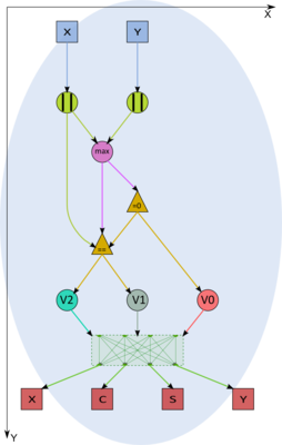
Figure 2. Choice of a method for calculating rotation parameters in vertices of type F1
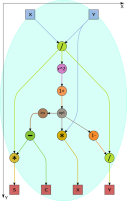
Figure 3. Calculation of the rotation parameters for various x and y in the vertex V2
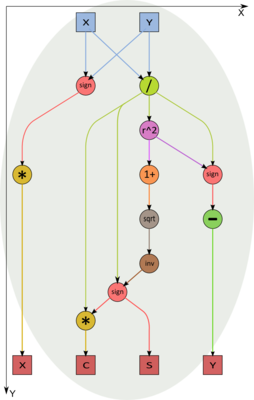
Figure 4. Calculation of the rotation parameters in the vertex V0 (the case of zero x and у)


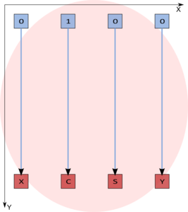
Figure 5. Calculation of the rotation parameters in the vertex V0 (the case of zero x and у)
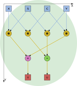
Figure 6. The inner graph of a vertex of type F2 with its input and output parameters: (u,v) = (c,s)(x,y)


1.8 Parallelization resource of the algorithm
In order to better understand the parallelization resource of Givens' decomposition of a matrix of order [math]n[/math], consider the critical path of its graph.
It is evident from the description of subgraphs that the macrovertex F1 (calculation of the rotation parameters) is much more "weighty" than the rotation vertex F2. Namely, the critical path of a rotation vertex consists of only one multiplication (there are four multiplications, but all of them can be performed in parallel) and one addition/subtraction (there are two operations of this sort, but they also are parallel). On the other hand, in the worst case, a macrovertex for calculating rotation parameters has the critical path consisting of a single square root calculation, two divisions, two multiplications, and two additions/subtractions.
According to a rough estimate, the critical path goes through [math]2n-3[/math] macrovertices of type F1 (calculating rotation parameters) and [math]n-1[/math] rotation macrovertices. Altogether, this yields a critical path passing through [math]2n-3[/math] square root extractions, [math]4n-6[/math] divisions, [math]5n-7[/math] multiplications, and the same number of additions/subtractions. In the macrograph shown in the figure, one of the critical paths consists of the passage through the upper line of F1 vertices (there are [math]n-1[/math] vertices) accompanied by the alternate execution of F2 and F1 ([math]n-2[/math] times) and the final execution of F2.
Thus, unlike in the serial version, square root calculations and divisions take a fairly considerable portion of the overall time required for the parallel variant. The presence of isolated square root calculations and divisions in some layers of the parallel form can also create other problems when the algorithm is implemented for a specific architecture. Consider, for instance, an implementation for PLDs. Other operations (multiplications and additions/subtractions) can be pipelined, which also saves resources. On the other hand, isolated square root calculations take resources that are idle most of the time.
In terms of the parallel form height, the Givens method is qualified as a linear complexity algorithm. In terms of the parallel form width, its complexity is quadratic.
1.9 Input and output data of the algorithm
Input data: dense square matrix [math]A[/math] (with entries [math]a_{ij}[/math]).
Size of the input data: [math]n^2[/math].
Output data: upper triangular matrix [math]R[/math] (in the serial version, the nonzero entries [math]r_{ij}[/math] are stored in the positions of the original entries [math]a_{ij}[/math]), unitary (or orthogonal) matrix [math]Q[/math] stored as the product of rotations (in the serial version, the rotation parameters [math]t_{ij}[/math] are stored in the positions of the original entries [math]a_{ij}[/math]).
Size of the output data: [math]n^2[/math].
1.10 Properties of the algorithm
It is clearly seen that the ratio of the serial to parallel complexity is quadratic, which is a good incentive for parallelization.
The computational power of the algorithm, understood as the ratio of the number of operations to the total size of the input and output data, is linear.
Within the framework of the chosen version, the algorithm is completely determined.
The roundoff errors in Givens (rotations) method grow linearly, as they also do in Householder (reflections) method.
2 Software implementation of the algorithm
2.1 Implementation peculiarities of the serial algorithm
In its simplest version, the QR decomposition of a real square matrix by Givens method can be written in Fortran as follows:
	DO  I = 1, N-1
		DO J = I+1, N
                    CALL PARAMS (A(I,I), A(J,I), C, S)
                    DO K = I+1, N
                       CALL ROT2D (C, S, A(I,K), A(J,K))
                    END DO
                END DO
	END DO
Suppose that the translator at hand competently implements operations with complex numbers. Then the rotation subroutine ROT2D can be written as follows:
	SUBROUTINE ROT2D (C, S, X, Y)
        COMPLEX Z
        REAL ZZ(2)
        EQUIVALENCE Z, ZZ
        Z = CMPLX(C, S)*CMPLX(X,Y)
        X = ZZ(1)
        Y = ZZ(2)
        RETURN
        END
or
	SUBROUTINE ROT2D (C, S, X, Y)
        ZZ = C*X - S*Y
        Y = S*X + C*Y
        X = ZZ
        RETURN
        END
(from the viewpoint of the algorithm graph, these subroutines are equivalent).
The subroutine for calculating the rotation parameters can have the following form:
	SUBROUTINE PARAMS (X, Y, C, S)
        Z = MAX (ABS(X), ABS(Y))
        IF (Z.EQ.0.) THEN
C OR (Z.LE.OMEGA) WHERE OMEGA - COMPUTER ZERO
            C = 1.
            S = 0.
        ELSE IF (Z.EQ.ABS(X))
            R = Y/X
            RR = R*R
            RR2 = SQRT(1+RR)
            X = X*RR2
            Y = (1-RR2)/R
            C = 1./RR2
            S = -C*R
        ELSE
            R = X/Y
            RR = R*R
            RR2 = SQRT (1+RR)
            X = SIGN(Y, X)*RR
            Y = R - SIGN(RR,R)
            S = SIGN(1./RR2, R)
            C = S*R
        END IF
        RETURN
        END
In the above implementation, the rotation parameter t is written to a vacant location (the entry of the modified matrix with the corresponding indices is known to be zero). This makes it possible to readily reconstruct rotation matrices (if required).
2.2 Possible methods and considerations for parallel implementation of the algorithm
On cluster-like supercomputers, a partitioning of an algorithm (with the usage of coordinate generalized schedule of the algorithm graph) and its distribution between different nodes (MPI) are fairly possible. At the same time, the inner parallelism in blocks will partially realize multi-core node capabilities (OpenMP) and even core superscalarity. This should be the aim of an implementation judging by the structure of the graph algorithm.
The structure of the graph makes one think that a good scalability can be attained, although, at the moment, this guess cannot be verified through concrete implementations. The favorable factors are a good (linear) nature of the critical path and a good coordinate structure of generalized schedule, which permits a good block partitioning of the algorithm graph.
An unexpected result was obtained by a search through the available program packages[3]. Most of old (serial) packages contain a subroutine for the QR decomposition via Givens method. By contrast, new packages, intended for parallel execution, perform the QR decomposition solely on the basis of Householder (reflections) method. Meanwhile, parallel properties of the latter are inferior to those of Givens method. We attribute this fact to that Householder method can easily be written in terms of BLAS-procedures, and it does not require loop reordering (except for the case where a partitioning is used; however, in this case, the coordinate rather than skewed loop partitioning is applied). On the other hand, some loop rewriting is needed for the parallel implementation of Givens method because skewed parallelism should be applied to achieve the maximum degree in its parallelization. Thus, we cannot assess the scalability of this algorithm implementations for the reason that no such implementations exist at the moment.
2.3 Run results
2.4 Conclusions for different classes of computer architecture
The module for calculating rotation parameters has a complicated logical structure. Therefore, we recommend the reader not to use PLDs as accelerators of universal processors for the reason that a significant part of their equipment will be idle. Certain difficulties are also possible on architectures with universal processors; however, the general structure of the algorithm makes it possible to expect a good performance from such architectures. For instance, on cluster-like supercomputers, a partitioning of the algorithm and its distribution between different nodes are fairly possible. At the same time, the inner parallelism in blocks will partially realize multi-core node capabilities and even core superscalarity.
3 References
- ↑ V.V. Voevodin, Yu.A. Kuznetsov. Matrices and Computations. Moscow, Nauka, 1984 (in Russian).
- ↑ V.V. Voevodin. Computational Foundations of Linear Algebra. Moscow, Nauka, 1977 (in Russian).
- ↑ A.V. Frolov, A.S. Antonov, Vl.V. Voevodin, A.M. Teplov. Comparison of different methods for solving the same problem on the basis of Algowiki methodology (in Russian) // Submitted to the conference "Parallel computational technologies (PaVT'2016)".