|
|
| (30 intermediate revisions by 3 users not shown) |
| Line 1: |
Line 1: |
| − | Primary authors of this description: [[:ru:Участник:Daryin|A.N.Daryin]], [[:ru:Участник:VadimVV|Vad.V.Voevodin]] ([[#Locality of data and computations|Section 2.2]]). | + | {{level-a}} |
| | + | Primary authors of this description: [[:ru:Участник:Daryin|A.N.Daryin]]. |
| | | | |
| | == Properties and structure of the algorithm == | | == Properties and structure of the algorithm == |
| Line 95: |
Line 96: |
| | | | |
| | === Implementation peculiarities of the serial algorithm === | | === Implementation peculiarities of the serial algorithm === |
| − |
| |
| − | === Locality of data and computations ===
| |
| − | ==== Locality of implementation ====
| |
| − | ===== Structure of memory access and a qualitative estimation of locality =====
| |
| − |
| |
| − | [[file:dijkstra_1.png|thumb|center|700px|Figure 1. Implementation of Dijkstra's algorithm. Overall memory access profile]]
| |
| − |
| |
| − | Fig.1 shows the memory address profile for an implementation of Dijkstra's algorithm. The first thing that is evident from this figure is a large separation of accesses. In particular, substantial regions above and below fragment 2 remain empty, while the accesses themselves form only small groups. This indicates low efficiency for two reasons: (a) there are practically no repeated accesses or such accesses occur at significant time intervals; (b) the distance between consecutive accesses may be fairly large.
| |
| − |
| |
| − | However, at closer examination, it may turn out that some areas have high locality and consist of a large number of accesses. Moreover, the overall profile contains several areas (fragments 1 and 2) in which the accesses are well localized. It is necessary to inspect individual areas in more detail.
| |
| − |
| |
| − | Let us consider fragment 1 (fig.2), within which accesses to two small arrays are performed. One can see that only about 500 elements are involved, and approximately 100 thousands accesses to these elements are done. The overall profile consist of about 120 thousands accesses. It follows that the overwhelming majority of accesses is performed exactly to the above elements.
| |
| − |
| |
| − | [[file:dijkstra_2.png|thumb|center|700px|Figure 2. Memory access profile, fragment 1]]
| |
| − |
| |
| − | Since, in this case, the number of elements is small, the locality is certainly sufficiently high regardless of the structure of the fragment. Figure 3 shows two subregions of fragment 1. Here, one can see that this fragment mainly consists of successive searches, and the data are often used repeatedly at not very large time intervals. All of this says that both the spatial and temporal localities of the fragment are high.
| |
| − |
| |
| − | [[file:dijkstra_3.png|thumb|center|700px|Figure 3. Profiles of two subregions of fragment 1 (shown in green in fig.2)]]
| |
| − |
| |
| − | Now, consider in more detail fragment 2 (fig.4). Here, accesses to another service array are performed, and the profile consists of two stages. At the first stage, accesses are scattered fairly chaotically, which reminds the random access. At the second stage, accesses form something like successive search. On the whole, such a profile has a very low temporal locality (because repeated accesses are completely or practically absent) and a rather low spatial locality (due to the random access at the first stage).
| |
| − |
| |
| − | Note that the number of elements involved is here greater than in fragment 1; however, the number of accesses is much smaller.
| |
| − |
| |
| − | [[file:dijkstra_4.png|thumb|center|500px|Figure 4. Memory access profile, fragment 2]]
| |
| − |
| |
| − | It remains to consider two arrays (the area between fragments 1 and 2 and the area below fragment 2). For these arrays, the patterns of accesses are in many ways similar; consequently, it is sufficient to examine one of them in more detail.
| |
| − |
| |
| − | Fragment 3 is shown in fig.5. This fragment represents a fairly large area, which does not allow us to analyze the profile up to individual accesses; however, this is not required here. It is evident that the profile is based on regions with successive searches of a small number of elements or similar searches performed with a small step. For instance, the largest region, distinguished in the fragment in yellow, consists of only two hundred accesses. The distance between different regions may be quite substantial. All of this says that the two arrays under discussion have a very low locality (both spatial and temporal).
| |
| − |
| |
| − | [[file:dijkstra_5.png|thumb|center|500px|Figure 5. Memory access profile, fragment 3]]
| |
| − |
| |
| − | On the whole, despite the positive contribution of the arrays in fragment 1, the locality of the overall profile should be rather low because, outside of this fragment, the data are used inefficiently.
| |
| − |
| |
| − | ===== Quantitative estimation of locality =====
| |
| − |
| |
| − | The basic fragment of the implementation used for obtaining quantitative estimates is given [http://git.parallel.ru/shvets.pavel.srcc/locality/blob/master/benchmarks/dijkstra/dijkstra.h here] (function Kernel). The start-up conditions are described [http://git.parallel.ru/shvets.pavel.srcc/locality/blob/master/README.md here].
| |
| − |
| |
| − | The first estimate is based on daps, which assesses the number of memory accesses (reads and writes) per second. Similar to flops, daps is used to evaluate memory access performance rather than locality. Yet, it is a good source of information, particularly for comparison with the results provided by the next estimate cvg.
| |
| − |
| |
| − | Fig.6 shows daps values for implementations of popular algorithms, sorted in ascending order (the higher the daps, the better the performance in general). One can see that the memory access performance is rather low. This is not surprising: implementations of graph algorithms have almost always a low efficiency because the data are accessed irregularly. We observed this while analyzing the memory access profile.
| |
| − |
| |
| − | [[file:dijkstra_daps.png|thumb|center|700px|Figure 6. Comparison of daps values]]
| |
| − |
| |
| − | The second characteristic – cvg – is intended for obtaining a more machine-independent locality assessment. It determines how often a program needs to pull data to cache memory. Accordingly, the smaller the cvg value, the less frequently data need to be pulled to cache, and the better the locality.
| |
| − |
| |
| − | Fig.7 shows the cvg values for the same set of implementations sorted in descending order (the smaller the cvg, the higher the locality in general). One can see that, in this case, the cvg value is well correlated with the performance estimate. It shows low locality, which conforms to the conclusions made in the qualitative assessment of locality.
| |
| − |
| |
| − |
| |
| − | [[file:dijkstra_cvg.png|thumb|center|700px|Figure 7. Comparison of cvg values]]
| |
| | | | |
| | === Possible methods and considerations for parallel implementation of the algorithm === | | === Possible methods and considerations for parallel implementation of the algorithm === |
| − | | + | === Run results === |
| − | === Scalability of the algorithm and its implementations === | |
| − | ==== Scalability of the algorithm ====
| |
| − | ==== Scalability of of the algorithm implementation ====
| |
| − | | |
| − | Let us study scalability for the parallel implementation of Dijkstra's algorithm in accordance with [[Scalability methodology|Scalability methodology]]. This study was conducted using the Lomonosov supercomputer of the <ref name="Lom">Воеводин Вл., Жуматий С., Соболев С., Антонов А., Брызгалов П., Никитенко Д., Стефанов К., Воеводин Вад. Практика суперкомпьютера «Ломоносов» // Открытые системы, 2012, N 7, С. 36-39.</ref> [http://parallel.ru/cluster Moscow University Supercomputing Center].
| |
| − | Набор и границы значений изменяемых [[Глоссарий#Параметры запуска|параметров запуска]] реализации алгоритма:
| |
| − | | |
| − | * число процессоров [4, 8 : 128] со значениями квадрата целого числа;
| |
| − | * размер графа [16000:64000] с шагом 16000.
| |
| − | | |
| − | На следующем рисунке приведен график [[Глоссарий#Производительность|производительности]] выбранной реализации алгоритма в зависимости от изменяемых параметров запуска.
| |
| − | | |
| − | [[file:Dijkstra perf.png|thumb|center|700px|Рисунок 8. Параллельная реализация алгоритма. Изменение производительности в зависимости от числа процессоров и размера области.]]
| |
| − | | |
| − | В силу особенностей параллельной реализации алгоритма производительность в целом достаточно низкая и с ростом числа процессов увеличивается медленно, а при приближении к числу процессов 128 начинает уменьшаться.
| |
| − | Это объясняется использованием коллективных операций на каждой итерации алгоритма и тем, что затраты на коммуникационные обмены существенно возрастают с ростом числа использованных процессов. Вычисления на каждом процессе проходят достаточно быстро и потому декомпозиция графа слабо компенсирует эффект от затрат на коммуникационные обмены.
| |
| − | | |
| − | [https://code.google.com/p/prir-dijkstra-mpi/source/browse/trunk/project/dijkstra_mpi.c Исследованная параллельная реализация на языке C]
| |
| − | | |
| − | === Dynamic characteristics and efficiency of the algorithm implementation ===
| |
| − | | |
| − | Для проведения экспериментов использовалась реализация алгоритма Дейкстры. Все результаты получены на суперкомпьютере "Ломоносов". Использовались процессоры Intel Xeon X5570 с пиковой производительностью в 94 Гфлопс, а также компилятор intel 13.1.0.
| |
| − | На рисунках показана эффективность реализации алгоритма Дейкстры на 32 процессах.
| |
| − | | |
| − | [[file:Dijkstra CPU User.png|thumb|center|700px|Рисунок 9. График загрузки CPU при выполнении алгоритма Дейкстры]]
| |
| − | | |
| − | На графике загрузки процессора видно, что почти все время работы программы уровень загрузки составляет около 50%. Это указывает на равномерную загруженность вычислениями процессоров, при использовании 8 процессов на вычислительный узел и без использования Hyper Threading.
| |
| − | | |
| − | [[file:Dijkstra Flops.png|thumb|center|700px|Рисунок 10. График операций с плавающей точкой в секунду при выполнении алгоритма Дейкстры]]
| |
| − | | |
| − | На Рисунке 10 показан график количества операций с плавающей точкой в секунду. На графике видна общая очень низкая производительность вычислений около 250 Kфлопс в пике и около 150 Кфлопс в среднем по всем узлам. Это указывает то, что в программе почти все вычисления производятся с целыми числами.
| |
| − | [[file:Dijkstra L1.png|thumb|center|700px|Рисунок 11. График кэш-промахов L1 в секунду при работе алгоритма Дейкстры]]
| |
| − |
| |
| − | На графике кэш-промахов первого уровня видно, что число промахов очень большое для нескольких ядер и находится на уровне 15 млн/сек (в пике до 60 млн/сек), что указывает на интенсивные вычисления в части процессов. В среднем по всем узлам значения значительно ниже (около 9 млн/сек). Это указывает на неравномерное распределение вычислений.
| |
| − | [[file:Dijkstra L3.png|thumb|center|700px|Рисунок 12. График кэш-промахов L3 в секунду при работе алгоритма Дейкстры]]
| |
| − | | |
| − | На графике кэш-промахов третьего уровня видно, что число промахов очень немного и находится на уровне 1,2 млн/сек, однако в среднем по всем узлам значения около 0,5 млн/сек. Соотношение кэш промахов L1|L3 для процессов с высокой производительностью доходит до 60, однако в среднем около 30. Это указывает на очень хорошую локальность вычислений как у части процессов, так и для всех в среднем, и это является признаком высокой производительности.
| |
| − | [[file:Dijkstra Mem Load.png|thumb|center|700px|Рисунок 13. График количества чтений из оперативной памяти при работе алгоритма Дейкстры]]
| |
| − | | |
| − | На графике обращений в память видна достаточно типичная картина для таких приложений. Активность чтения достаточно низкая, что в совокупности с низкими значениями кэш-промахов L3 указывает на хорошую локальность. Хорошая локальность приложения так же указывает на то, что значения около 1 млн/сек для задачи является результатом высокой производительности вычислений, хотя и присутствует неравномерность между процессами.
| |
| − | [[file:Dijkstra Mem Store.png|thumb|center|700px|Рисунок 14. График количества записей в оперативную память при работе алгоритма Дейкстры]]
| |
| − | | |
| − | На графике записей в память видна похожая картина неравномерности вычислений, при которой одновременно активно выполняют запись только несколько процессов. Это коррелирует с другими графиками выполнения. Стоит отметить, достаточно низкое число обращений на запись в память. Это указывает на хорошую организацию вычислений, и достаточно эффективную работу с памятью.
| |
| − | [[file:Dijkstra Inf DATA.png|thumb|center|700px|Рисунок 15. График скорости передачи по сети Infiniband в байт/сек при работе алгоритма Дейкстры]]
| |
| − | | |
| − | На графике скорости передачи данных по сети Infiniband наблюдается достаточно высокая скорость передачи данных в байтах в секунду. Это говорит о том, что процессы между собой обмениваются интенсивно и вероятно достаточно малыми порциями данных, потому как производительность вычислений высока. Стоит отметить, что скорость передачи отличается между процессами, что указывает на дисбаланс вычислений.
| |
| − | [[file:Dijkstra Inf PCKTS.png|thumb|center|700px|Рисунок 16. График скорости передачи по сети Infiniband в пакетах/сек при работе алгоритма Дейкстры]]
| |
| − | | |
| − | На графике скорости передачи данных в пакетах в секунду наблюдается крайне высокая интенсивность передачи данных выраженная в пакетах в секунду. Это говорит о том, что, вероятно, процессы обмениваются не очень существенными объемами данных, но очень интенсивно. Используются коллективные операции на каждом шаге с небольшими порциями данных, что объясняет такую картину. Так же наблюдается почти меньший дизбаланс между процессами чем наблюдаемый в графиках использования памяти и вычислений и передачи данных в байтах/сек. Это указывает на то, что процессы обмениваются по алгоритму одинаковым числом пакетов, однако получают разные объемы данных и ведут неравномерные вычисления.
| |
| − | [[file:Dijkstra Load ABG.png|thumb|center|700px|Рисунок 17. График числа процессов, ожидающих вхождения в стадию счета (Loadavg), при работе алгоритма Дейкстры]]
| |
| − | На графике числа процессов, ожидающих вхождения в стадию счета (Loadavg), видно, что на протяжении всей работы программы значение этого параметра постоянно и приблизительно равняется 8. Это свидетельствует о стабильной работе программы с загруженными вычислениями всеми узлами. Это указывает на очень рациональную и статичную загрузку аппаратных ресурсов процессами. И показывает достаточно хорошую эффективность выполняемой реализации.
| |
| − | В целом, по данным системного мониторинга работы программы можно сделать вывод о том, что программа работала достаточно эффективно, и стабильно. Использование памяти очень интенсивное, а использование коммуникационной среды крайне интенсивное, при этом объемы передаваемых данных не являются высокими. Это указывает на требовательность к латентности коммуникационной среды алгоритмической части программы.
| |
| − | Низкая эффективность связана судя по всему с достаточно высоким объемом пересылок на каждом процессе, интенсивными обменами сообщениями.
| |
| − | | |
| | === Conclusions for different classes of computer architecture === | | === Conclusions for different classes of computer architecture === |
| − | === Existing implementations of the algorithm ===
| |
| − |
| |
| − | * C++: [http://www.boost.org/libs/graph/doc/ Boost Graph Library] (функции <code>[http://www.boost.org/libs/graph/doc/dijkstra_shortest_paths.html dijkstra_shortest_paths]</code>, <code>[http://www.boost.org/libs/graph/doc/dijkstra_shortest_paths_no_color_map.html dijkstra_shortest_paths_no_color_map]</code>), сложность <math>O(m + n \ln n)</math>.
| |
| − | * C++, MPI: [http://www.boost.org/libs/graph_parallel/doc/html/index.html Parallel Boost Graph Library]:
| |
| − | ** функция <code>[http://www.boost.org/libs/graph_parallel/doc/html/dijkstra_shortest_paths.html#eager-dijkstra-s-algorithm eager_dijkstra_shortest_paths]</code> – непосредственная реализация алгоритма Дейкстры;
| |
| − | ** функция <code>[http://www.boost.org/libs/graph_parallel/doc/html/dijkstra_shortest_paths.html#crauser-et-al-s-algorithm crauser_et_al_shortest_paths]</code> – реализация алгоритма Дейкстры в виде алгоритма из статьи Краузера и др.<ref>Crauser, A, K Mehlhorn, U Meyer, and P Sanders. “A Parallelization of Dijkstra's Shortest Path Algorithm,” Proceedings of Mathematical Foundations of Computer Science / Lecture Notes in Computer Science, 1450:722–31, Berlin, Heidelberg: Springer, 1998. doi:10.1007/BFb0055823.</ref>
| |
| − | * Python: [https://networkx.github.io NetworkX] (функция <code>[http://networkx.github.io/documentation/networkx-1.9.1/reference/generated/networkx.algorithms.shortest_paths.weighted.single_source_dijkstra.html single_source_dijkstra]</code>).
| |
| − | * Python/C++: [https://networkit.iti.kit.edu NetworKit] (класс <code>[https://networkit.iti.kit.edu/data/uploads/docs/NetworKit-Doc/python/html/graph.html#networkit.graph.Dijkstra networkit.graph.Dijkstra]</code>).
| |
| | | | |
| | == References == | | == References == |
Primary authors of this description: A.N.Daryin.
1 Properties and structure of the algorithm
1.1 General description of the algorithm
Dijkstra's algorithm[1] was designed for finding the shortest paths between nodes in a graph. For a given weighted digraph with nonnegative weights, the algorithm finds the shortest paths between a singled-out source node and the other nodes of the graph.
Dijkstra's algorithm (using Fibonacci heaps [2]) is executed in [math]O(m + n \ln n)[/math] time and, asymptotically, is the fastest of the known algorithms for this class of problems.
1.2 Mathematical description of the algorithm
Let [math]G = (V, E)[/math] be a given graph with arc weights [math]f(e)[/math] and the single-out source node [math]u[/math]. Denote by [math]d(v)[/math] the shortest distance between the source [math]u[/math] and the node [math]v[/math].
Suppose that one has already calculated all the distances not exceeding a certain number [math]r[/math], that is, the distances to the nodes in the set [math]V_r = \{ v \in V \mid d(v) \le r \}[/math]. Let
- [math]
(v, w) \in \arg\min \{ d(v) + f(e) \mid v \in V, e = (v, w) \in E \}.
[/math]
Then [math]d(w) = d(v) + f(e)[/math] and [math]v[/math] lies on the shortest path from [math]u[/math] to [math]w[/math].
The values [math]d^+(w) = d(v) + f(e)[/math], where [math]v \in V_r[/math], [math]e = (v, w) \in E[/math], are called expected distances and are upper bounds for the actual distances: [math]d(w) \le d^+(w)[/math].
Dijkstra's algorithm finds at each step the node with the least expected distance, marks this node as a visited one, and updates the expected distances to the ends of all arcs outgoing from this node.
1.3 Computational kernel of the algorithm
The basic computations in the algorithm concern the following operations with priority queues:
- retrieve the minimum element (
delete_min);
- decrease the priority of an element (
decrease_key).
1.4 Macro structure of the algorithm
Pseudocode of the algorithm:
Input data:
  graph with nodes V and arcs E with weights f(e);
  source node u.
Output data: distances d(v) to each node v ∈ V from the node u.

Q := new priority queue
for each v ∈ V:
    if v = u then d(v) := 0 else d(v) := ∞
    Q.insert(v, d(v))

while Q ≠ ∅:
    v := Q.delete_min()
    for each e = (v, w) ∈ E:
        if d(w) > d(v) + f(e):
            d(w) := d(v) + f(e)
            Q.decrease_key(w, d(w))
1.5 Implementation scheme of the serial algorithm
A specific implementation of Dijkstra's algorithm is determined by the choice of an algorithm for priority queues. In the simplest case, it can be an array or a list in which search for the minimum requires the inspection of all nodes. Algorithms that use heaps are more efficient. The variant using Fibonacci heaps [2] has the best known complexity estimate.
It is possible to implement the version in which nodes are added to the queue at the moment of the first visit rather than at the initialization stage.
1.6 Serial complexity of the algorithm
The serial complexity of the algorithm is [math]O(C_1 m + C_2n)[/math], where
- [math]C_1[/math] is the number of operations for decreasing the distance to a node;
- [math]C_2[/math] is the number of operations for calculating minima.
The original Dijkstra's algorithm used lists as an internal data structure. For such lists, [math]C_1 = O(1)[/math], [math]C_2 = O(n)[/math], and the total complexity is [math]O(n^2)[/math].
If Fibonacci heaps [2] are used, then the time for calculating a minimum decreases to [math]C_2 = O(\ln n)[/math] and the total complexity is [math]O(m + n \ln n)[/math], which, asymptotically, is the best known result for this class of problems.
1.7 Information graph
Figure 1 shows the graph of the basic implementation of Dijkstra's algorithm based on lists or arrays.
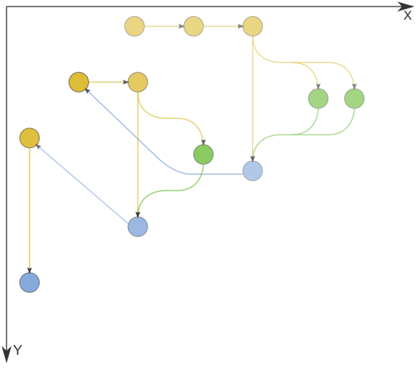
Figure 1. Information graph of Dijkstra's algorithm. The input and output data are not shown. n=3. Comparison operations, operations for changing node labels, and node labeling operations are indicated in yellow, green, and blue, respectively.
1.8 Parallelization resource of the algorithm
Dijkstra's algorithm admits an efficient parallelization [3] Its average execution time is [math]O(n^{1/3}\ln n)[/math], and the computational complexity is [math]O(n \ln n + m)[/math].
The algorithm of Δ-stepping can be regarded as a parallel version of Dijkstra's algorithm.
1.9 Input and output data of the algorithm
Input data: weighted graph [math](V, E, W)[/math] ([math]n[/math] nodes [math]v_i[/math] and [math]m[/math] arcs [math]e_j = (v^{(1)}_{j}, v^{(2)}_{j})[/math] with weights [math]f_j[/math]), source node [math]u[/math].
Size of input data: [math]O(m + n)[/math].
Output data (possible variants):
- for each node [math]v[/math] of the original graph, the last arc [math]e^*_v = (w, v)[/math] lying on the shortest path from [math]u[/math] to [math]v[/math] or the corresponding node [math]w[/math];
- for each node [math]v[/math] of the original graph, the summarized weight [math]f^*(v)[/math] of the shortest path from [math]u[/math] to [math]v[/math].
Size of output data: [math]O(n)[/math].
1.10 Properties of the algorithm
2 Software implementation of the algorithm
2.1 Implementation peculiarities of the serial algorithm
2.2 Possible methods and considerations for parallel implementation of the algorithm
2.3 Run results
2.4 Conclusions for different classes of computer architecture
3 References
- ↑ Dijkstra, E W. “A Note on Two Problems in Connexion with Graphs.” Numerische Mathematik 1, no. 1 (December 1959): 269–71. doi:10.1007/BF01386390.
- ↑ 2.0 2.1 2.2 Fredman, Michael L, and Robert Endre Tarjan. “Fibonacci Heaps and Their Uses in Improved Network Optimization Algorithms.” Journal of the ACM 34, no. 3 (July 1987): 596–615. doi:10.1145/28869.28874.
- ↑ Crauser, A, K Mehlhorn, U Meyer, and P Sanders. “A Parallelization of Dijkstra's Shortest Path Algorithm,” Proceedings of Mathematical Foundations of Computer Science / Lecture Notes in Computer Science, 1450:722–31, Berlin, Heidelberg: Springer, 1998. doi:10.1007/BFb0055823.
