Forward substitution

Primary authors of this description: A.V.Frolov, Vad.V.Voevodin (Section 2.2), A.M. Teplov (Section 2.4)

1 Properties and structure of the algorithm

1.1 General description of the algorithm

Forward substitution is the process of solving a system of linear algebraic equations (SLAE) [math]Lx = y[/math] with a lower triangular coefficient matrix [math]L[/math]. The matrix [math]L[/math] is a factor of the matrix [math]A[/math] and results from either the [math]LU[/math]-decomposition of the latter obtained by any of numerous ways (such as simple Gaussian elimination or Gaussian elimination with pivoting or compact schemes of Gaussian elimination) or other types of decomposition. The triangular form of [math]L[/math] ensures that the process of solving a SLAE is a modification of the general substitution method and this process can be described by simple formulas.

In [1], the process of solving a SLAE with a lower triangular coefficient matrix was named the back substitution. It was also noted in [1] that, in the literature, back substitution is usually regarded as solving a SLAE with a right triangular matrix, whereas the solution of left triangular systems is called the forward substitution. We adopt this nomenclature in order to avoid using identical names for different algorithms. Furthermore, unlike the forward substitution treated here, the back substitution, as presented in this algorithmic encyclopedia, is at the same time one of the stages in Gaussian elimination for solving SLAEs, namely, the final stage of this method.

Nevertheless, the structure of the forward substitution for a nonsingular left triangular matrix is virtually identical to the structure of the back substitution. Here, we consider the case where [math]L[/math] is a matrix obtained from a Gauss-like decomposition and, hence, [math]L[/math] has unit diagonal entries.

1.2 Mathematical description of the algorithm

Input data: left triangular matrix [math]L[/math] (with entries [math]l_{ij}[/math]), right-hand side vector [math]b[/math] (with components [math]b_{i}[/math]).

Output data: solution vector [math]y[/math] (with components [math]y_{i}[/math]).

Formulas of the method:

[math] \begin{align} y_{1} & = b_{1} \\ y_{i} & = b_{i} - \sum_{j = 1}^{i-1} l_{ij} y_{j}, \quad i \in [2, n]. \end{align} [/math]

There exists also a block version of the method; however, this description treats only the pointwise version.

1.3 Computational kernel of the algorithm

The computational kernel of the forward substitution could be compiled of repeated dot products of the rows of [math]L[/math] and the already determined portions of the vector [math]y[/math] (there are on the whole [math]n-1[/math] products) :

[math] \sum_{j = 1}^{i-1} l_{ij} y_{j} [/math]

Depending on the problem requirements, these products are calculated with or without using the accumulation mode. Then they are subtracted from the corresponding components of the vector [math]b[/math], and the results are divided by the corresponding diagonal entries of [math]L[/math]. This scheme is, however, not used in domestic implementations, even in serial ones. In these implementations, sums of the type

[math] b_{i} - \sum_{j = 1}^{i-1} l_{ij} y_{j} [/math]

(and dot products are exactly such sums) are not calculated according to the rule "first, find the dot product and then subtract it from the given element". Instead, the componentwise products, which are summands of the dot product, are one by one subtracted from this element. Consequently, the calculation of the expressions

[math] b_{i} - \sum_{j = 1}^{i-1} l_{ij} y_{j} [/math]

rather than dot products should be regarded as the computational kernel of the forward substitution. Depending on the problem requirements, these expressions are calculated with or without using the accumulation mode.

1.4 Macro structure of the algorithm

As already noted in the description of the computational kernel, the basic part of the forward substitution is compiled of repeated calculations of the sums

[math] b_{i} - \sum_{j = 1}^{i-1} l_{ij} y_{j} [/math]

(there are on the whole [math]n-1[/math] sums). These calculations are performed with or without using the accumulation mode.

1.5 Implementation scheme of the serial algorithm

To make the order of calculations clearer, rewrite the formulas of the method as follows.

1. [math]y_{1} = b_{1}[/math]

Then, for [math]i[/math] increasing from [math]2[/math] to [math]n[/math], do

2. [math]y_{i} = b_{i} - \sum_{j = 1}^{i-1} l_{ij} y_{j}[/math]

We emphasize that sums of the form [math]b_{i} - \sum_{j = 1}^{i-1} l_{ij} y_{j}[/math] are calculated in the accumulation mode by subtracting from [math]b_{i}[/math] the products [math]l_{ij} y_{j}[/math]for [math]j[/math] increasing from [math]1[/math] to [math]i-1[/math]. Any other order of summation makes the parallel properties of the algorithm much worse.

1.6 Serial complexity of the algorithm

The forward substitution of order n in its serial (that is, the fastest) version requires

• [math]\frac{n^2-n}{2}[/math] multiplications and the same number of additions (subtractions).

The use of accumulation requires that multiplications and subtractions be done in the double precision mode (or such procedures as the Fortran function DPROD be used). This increases the computation time for performing the forward substitution.

In terms of serial complexity, the forward substitution is qualified as a quadratic complexity algorithm.

1.7 Information graph

We describe the graph of the algorithm both analytically and graphically.

Forward substitution

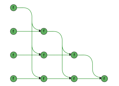
The graph of forward substitution consists of a single group of vertices placed at integer nodes of a two-dimensional domain. The corresponding operation is [math]a-bc[/math].

The natural coordinates of this domain are as follows:

• [math]i[/math] changes from [math]2[/math] to [math]n[/math], taking all the integer values in this range;
• [math]j[/math] changes from [math]1[/math] to [math]i-1[/math], taking all the integer values in this range.

The arguments of the operation are as follows:

• [math]a[/math] is:
  • the element [math]b_{i}[/math] of the input data if [math]j = 1[/math];
  • the result of performing the operation corresponding to the vertex with coordinates [math]i, j-1[/math] if [math]j \gt 1[/math];
• [math]b[/math] is the element [math]l_{ij}[/math] of the input data;
• [math]c[/math] is:
  • the element [math]b_{1}[/math] of the input data if [math]j = 1[/math];
  • the result of performing the operation corresponding to the vertex with coordinates [math]j, j-1[/math] if [math]j \gt 1[/math].

The result of performing the operation is:

• an intermediate data item if [math]j \lt i-1[/math] ;
• an output data item if [math]j = i-1[/math] .

The graph described can be seen in the figure corresponding to the case [math]n = 5[/math]. The vertices are depicted in green. The supplies of the input data from the vector [math]b[/math] to the vertices of the left column and from the matrix [math]L[/math] to all the vertices are not shown in the figure.

1.8 Parallelization resource of the algorithm

The parallel version of the forward substitution of order n requires that the following layers be successively performed:

• [math]n - 1[/math] layers involving multiplications and additions / subtractions. (The number of operations changes linearly from [math]1[/math] to [math]n-1[/math].)

The use of accumulation requires that multiplications and subtractions be done in the double precision mode. For the parallel version, this implies that virtually all the intermediate calculations in the algorithm must be performed in double precision if the accumulation option is used. Unlike the situation with the serial version, this results in a certain increase in the required memory size.

In terms of the parallel form height, the forward substitution is qualified as a linear complexity algorithm. Its complexity is also linear in terms of the parallel form width.

1.9 Input and output data of the algorithm

Input data: left triangular matrix [math]L[/math] (with entries [math]l_{ij}[/math]), right-hand side vector [math]b[/math] (with components [math]b_{i}[/math]).

Size of the input data : [math]\frac{n (n + 1)}{2}[/math] (since [math]L[/math] is triangular and has unit diagonal entries, it suffices that only its subdiagonal entries be stored).

Output data : solution vector [math]y[/math] (with components [math]y_{i}[/math]).

Size of the output data: [math]n~.[/math]

1.10 Properties of the algorithm

It is clear that, in the case of unlimited resources, the ratio of the serial to parallel complexity is linear (since this is the ratio of the quadratic to linear complexity).

The computational power of the forward substitution, understood as the ratio of the number of operations to the total size of the input and output data, is only a constant.

In this version, the algorithm of forward substitution is completely determined. We do not consider any other order of performing operations because, otherwise, the structure of the algorithm would radically change and the parallel complexity would be quadratic.

2 Software implementation of the algorithm

2.1 Implementation peculiarities of the serial algorithm

In its simplest form, the forward substitution algorithm in Fortran can be written as follows:

        Y(1) = B(1) 
	DO  I = 2, N-1
		S = B(I)
		DO  J = 1, I-1
			S = S - DPROD(L(I,J), Y(J))
		END DO		
	END DO

In this case, the [math]S[/math] variable must be of the double type to implement the accumulation mode.

2.2 Locality of data and computations

2.2.1 Locality of implementation

2.2.1.1 Structure of memory access and a qualitative estimation of locality

Figure 12.1. Gaussian forward decomposition method of a system of linear equations. Overall memory call profile

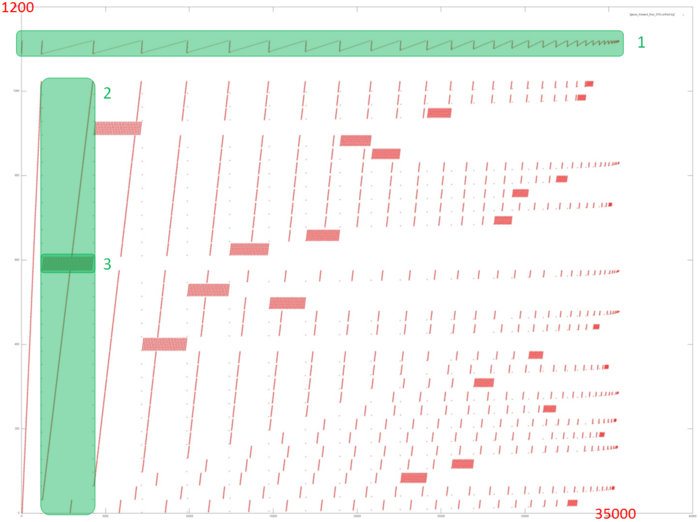
Figure 12.1 shows the memory call profile for the forward Gaussian decomposition of a system of linear equations. Like the source code, the figure shows that the program involves two primary arrays of data: calls to elements of the first array are marked in green (Fragment 1); all other calls are to elements of the second array. It is clear that the program has a complex profile. The main conclusion that can be made from this figure is the iterative nature of the profile, where each subsequent iteration contains fewer calls. This is particularly clear from Fragment 1.

Next, as you know, the Gaussian method discards one line from the linear system of equations with each iteration. This is also clear from Figure 12.1: each iteration (one of which is selected as Fragment 2) consists of a series of memory calls related to the line being discarded (Fragment 3), after which these elements are no longer addressed. It can also be seen that fragments similar to Fragment 3 are becoming smaller with each subsequent iteration, both in terms of the number of calls and number of elements addressed.

However, this general picture is very difficult for providing a qualitative assessment of data locality. Let’s move to a more detailed view of Fragment 1, which corresponds to the access to one of the two data arrays in memory.

Figure 12.2. Fragment 1 (First array memory call profile)

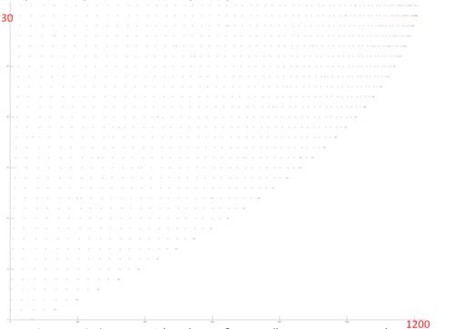
Figure 12.2 shows a detailed view of Fragment 1, highlighted in green in Figure 12.1. The picture looks curious: based on Figure 12.1, the impression was that this profile consisted of two different cycles of iterations, with the first cycle iterations being substantially shorter than second cycle iterations. In fact, Figure 12.2 shows that the profile consists of the same type of iterations, reading the array elements sequentially. With each subsequent iteration, the element with the smallest index is discarded. The illusion of two different cycles is created solely by the number of calls to the other array – when the number of such calls is high, the iteration for this fragment looks longer. Fragment 1 (as shown in Figure 12.2) has only about 1,200 memory calls, while the entire profile has 34,000 calls. That is, the first array accounts for just 3.5% of all memory calls in the program.

Since this profile is based on a sequential search through the array elements, we can say the fragment has high spatial locality. And since there are many iterations searching through array elements, it is clear that temporal locality is also high.

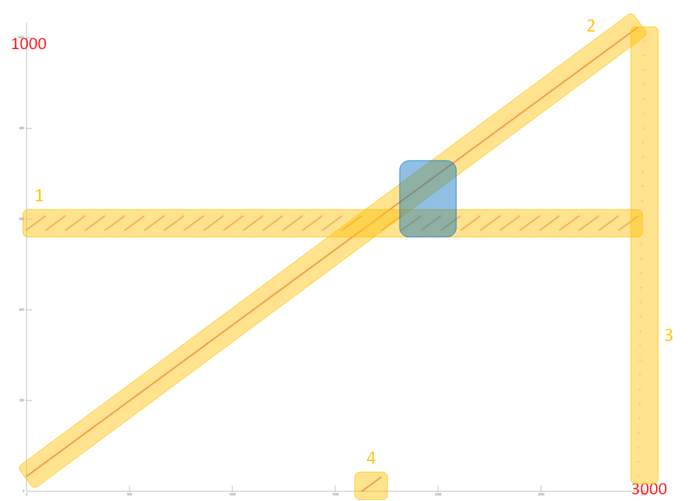
Now let’s review the memory call profile for the second array, which is substantially larger and more complex than the first profile. Figure 12.3 shows a detailed view of Fragment 2 as highlighted in Figure 12.1. This fragment consists of four parts, highlighted in orange.

Figure 12.3. Fragment 2 (an iteration of memory calls to the second array)

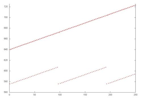
Part 1 looks like a cyclic sequential search through a small part of the array elements, and a closer look shows this is indeed the case. Figure 12.4 shows a close-up of Fragment 2 which is highlighted in blue in Figure 12.3. This close-up also shows that Part 2 is nearly identical to a sequential search of all elements of this array. Thus, both parts have very high spatial locality (due to the sequential search). Part 1 also has high temporal locality, as the search is repeated in a cycle, unlike part 2, where each element is only addressed once.

Part 3 consists of only a few memory calls, and represents a sequential search of all array elements with a very large interval – much larger than in Part 2. In this case, due to the high interval, spatial locality is low and there is no temporal locality either as the search is only done once.

Part 4 represents another sequential search through a small part of the array, the size of which equals the number of discarded array elements; the closer to the end of the profile, the more memory calls are there in part 4. This part has the same locality properties as Part 2. The only difference is in the size, but it does not affect the locality much.

When viewing Fragment 2 in general, the main impact comes from parts 1 and 2; therefore we can say this fragment has high temporal and spatial locality. However, with subsequent iterations (see Figure 12.1) locality will generally be decreasing as each iteration discards several elements.

Figure 12.4. Close-up view of Fragment 2

2.2.1.2 Quantitative estimation of locality

The key implementation fragment which was used to obtain a quantitative assessment is presented here (Kernel1 function). Launch conditions are described here.

The first estimate is based on daps, which assesses the number of memory access operations (reads and writes) per second. Similar to flops, this tool is used to evaluate memory access performance, rather than locality. But it is still a good source of information, particularly in combination with the next estimate – cvg.

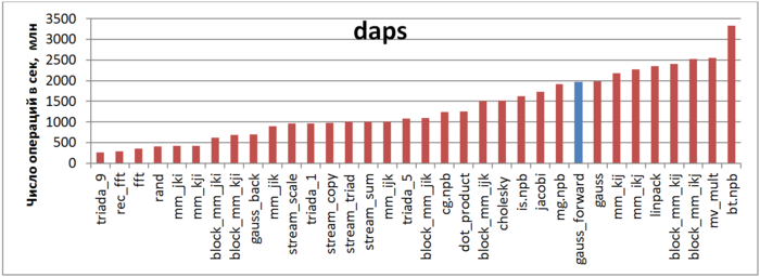
Figure 12.5 shows the daps values for various implementations of common algorithms sorted in ascending order (larger daps values generally mean higher performance). You can see that the blue column, which corresponds to the Forward Guassian method, is located in the right part of the chart indicating high performance, a little lower than the Linpak test performance. It should also be noted that the daps value for this task is almost equal to the daps value for the entire Gaussian method (“gauss” column), which combines the forward and reverse methods. This is due to the fact that reverse method has a much lower number of memory calls than forward method, so its impact is limited.

Figure 12.5. Comparison of daps values

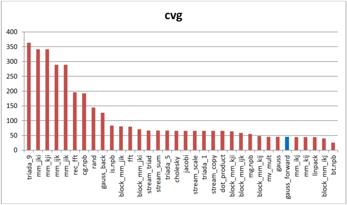
The second tool – cvg – is intended to obtain a more machine-independent locality assessment. It determines how often a program needs to pull data to cache memory. Respectively, the smaller the cvg value, the less frequently data needs to be called to cache, and the better the locality.

Figure 12.6 shows cvg values for the same set of implementations, sorted in descending order (lower cvg generally means higher locality). You can see that according to this assessment, just as with daps, the forward Gaussian method has high locality. The Linpak test offers comparable results as well. Interestingly, the ranking for the forward method and a combination of the forward and reverse methods together (“gauss” column) are almost the same.

Figure 12.6. Comparison of cvg values

2.4 Scalability of the algorithm and its implementations

2.4.2 Scalability of of the algorithm implementation

Figure 1. Scalability of the forward Gaussian method parallel implementation. Maximum performance.

Figure 2. Scalability of the forward Gaussian method parallel implementation. Maximum efficiency.

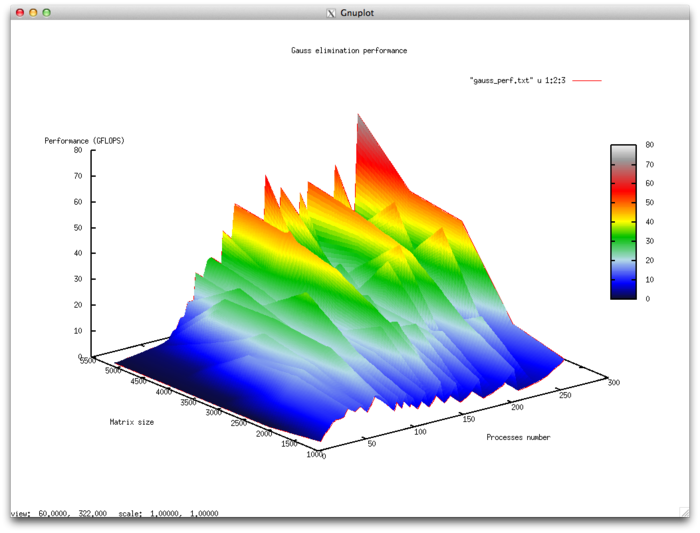
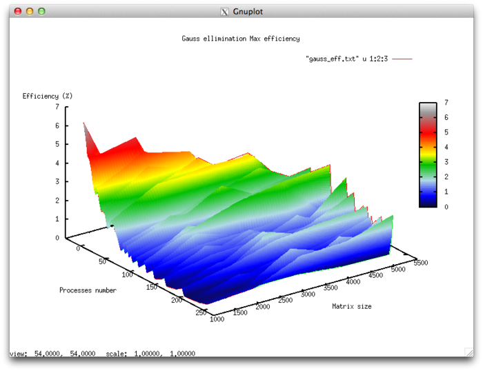
The set of variable launch parameters for the algorithm implementation and limits for the algorithm parameter values:

• Number of processors [4 : 256]
• Matrix size [1024 : 5120]

Efficiency of algorithm implementation execution

• Minimum efficiency 0.11%
• Maximum efficiency 6.65%

Scalability evaluation:

• By the number of processes: -0.000101 – as the number of processes increases, overall efficiency declines in the area considered, even though not as intensely as when the task size increases. Considering the 6.5% difference between the maximum and minimum efficiency, we can conclude that the efficiency reduction is most likely quite uniform within the area considered. The efficiency reduction is explained by the fact that as computing power grows, so does the volume of data sent back and forth. Some efficiency increases can be present at all matrix sizes considered. This can be due to increases in the program’s computational complexity, which results in overall efficiency growth given fixed overhead costs for organizing parallel computing.
• By task size: –0.0674 – as the task size grows, efficiency generally decreases within the area considered. This can be explained by the fact that as the task size is increased, so does the overhead cost of organizing parallel computing. As efficiency reduction along this axis is more intense than with an increase in the number of processes, the efficiency drop will most likely be more intense with a smaller number of processes than in existing areas of increasing efficiency with a larger number of processes.
• In both directions: –6.621e-05 – as both computational complexity and the number of processes increase throughout the area considered, efficiency falls, but at a very low rate. Given that the difference between maximum and minimum efficiency at the given range of parameter values is under 6.5%, this shows that if there are any areas on the surface with a very intense change of efficiency, they will have a small area. On the rest of the surface, efficiency changes are small and are located at about the same level.

Parallel implementation examined in C