Difference between revisions of "Gaussian elimination, compact scheme for tridiagonal matrices, serial variant"
| [unchecked revision] | [quality revision] |
| (19 intermediate revisions by one other user not shown) | |||
| Line 8: | Line 8: | ||
}} | }} | ||
| − | Main | + | Main author: [[:ru:Участник:Frolov|Alexey Frolov]] |
== Properties and structure of the algorithm == | == Properties and structure of the algorithm == | ||
| Line 14: | Line 14: | ||
=== General description of the algorithm === | === General description of the algorithm === | ||
| − | '''Сompact scheme for Gaussian elimination, as applied to tri-diagonal matrices'''<ref> | + | '''Сompact scheme for Gaussian elimination, as applied to tri-diagonal matrices'''<ref>Voevodin V.V. Computational foundations of linear algebra Moscow: Nauka, 1977.</ref><ref>Voevodin V.V., Kuznetsov Yu.A. Matrices and computations, Moscow: Nauka, 1984.</ref>, calculates the <math>LU</math> decomposition of a tri-diagonal matrix |
{{Template:Standard tridiagonal matrix}} | {{Template:Standard tridiagonal matrix}} | ||
| Line 23: | Line 23: | ||
{{Template:U2dCommon}}. | {{Template:U2dCommon}}. | ||
| − | The choice of fixed values for the diagonal entries of <math>L</math> makes all the nonzero entries in the decomposition uniquely determined (up to round-off errors). The compact scheme provides natural formulas for these entries. The <math>LU</math> decomposition of a tri-diagonal matrix is a particular case of the general [[ | + | The choice of fixed values for the diagonal entries of <math>L</math> makes all the nonzero entries in the decomposition uniquely determined (up to round-off errors). The compact scheme provides natural formulas for these entries. The <math>LU</math> decomposition of a tri-diagonal matrix is a particular case of the general [[Compact scheme for Gaussian elimination|compact scheme for Gaussian elimination]]. However, the specificity of the tri-diagonal case drastically changes the characteristics of the algorithm compared to the compact scheme for dense matrices. |
=== Mathematical description of the algorithm === | === Mathematical description of the algorithm === | ||
| Line 78: | Line 78: | ||
<div class="thumbinner" style="width:{{#expr: 2 * (500 + 35) + 3 * (3 - 1) + 8}}px"> | <div class="thumbinner" style="width:{{#expr: 2 * (500 + 35) + 3 * (3 - 1) + 8}}px"> | ||
<gallery widths=500px heights=500px> | <gallery widths=500px heights=500px> | ||
| − | File:3dLU.png| | + | File:3dLU.png|Figure 1. Graph of the algorithm. The input and output data are not shown. / - division, * - multiplication, - - subtraction. |
| − | File:3dLU_input.png| | + | File:3dLU_input.png|Figure 2. Graph of the algorithm. The input data are shown. / - division, * - multiplication, - - subtraction. |
</gallery> | </gallery> | ||
</div> | </div> | ||
</div> | </div> | ||
| − | + | One can see from Figure 1, where one of the operations is decomposed into two constituents, that the information graph is purely serial. | |
=== Parallelization resource of the algorithm === | === Parallelization resource of the algorithm === | ||
| − | + | In order to factorize a tri-diagonal matrix of order n by using the compact scheme of Gaussian elimination, one should perform | |
| − | * <math>n-1</math> | + | * <math>n-1</math> layers of division, |
| − | * <math>n-1</math> | + | * <math>n-1</math> layers of multiplication, |
| − | * <math>n-1</math> | + | * <math>n-1</math> layers of addition (subtraction). |
| − | + | Each layer consists of a single operation. Hence, in terms of the parallel form height, the compact scheme of Gaussian elimination for factoring tri-diagonal matrices, in its serial version, is a ''linear complexity'' algorithm. The layer width is everywhere equal to 1. Thus, the entire algorithm is an all-over bottleneck. | |
=== Input and output data of the algorithm === | === Input and output data of the algorithm === | ||
| − | ''' | + | '''Input data''': tri-diagonal matrix <math>A</math> (with entries <math>a_{ij}</math>). |
| − | ''' | + | '''Size of the input data''': <math>3n-2</math>. Different implementations may store the information differently for economy reasons. For instance, each diagonal of the matrix can be stored by a separate row of the array. |
| − | ''' | + | '''Output data''': lower bi-diagonal matrix <math>L</math> (with entries <math>l_{ij}</math>, where <math>l_{ii}=1</math>) and upper bi-diagonal matrix <math>U</math> (with entries <math>u_{ij}</math>). |
| − | ''' | + | '''Size of the output data''' is formally <math>3n-2</math>. However, since <math>n</math> items in the input and output data are identical, actually only <math>2n-2</math> items are calculated. |
=== Properties of the algorithm === | === Properties of the algorithm === | ||
| − | + | It is clear that, in the case of unlimited resources, the ratio of the serial to parallel complexity is '''one''' (that is, the algorithm is non-parallelizable). | |
| − | + | The computational power of the algorithm, understood as the ratio of the number of operations to the total size of the input and output data, is only a | |
| + | '''constant''' (the number of arithmetic operations is the same as the size of the data). | ||
| − | + | The algorithm is completely determined. | |
| − | [[ | + | The [[Glossary#Equivalent_perturbation|equivalent perturbation]] <math>M</math> of the algorithm does not exceed the perturbation <math>\delta A</math> that results from inputting the data into memory: |
<math> | <math> | ||
||M||_{E} \leq ||\delta A||_{E} | ||M||_{E} \leq ||\delta A||_{E} | ||
| Line 123: | Line 124: | ||
=== Implementation peculiarities of the serial algorithm === | === Implementation peculiarities of the serial algorithm === | ||
| − | + | In its simplest version, the algorithm can be written in Fortran as follows: | |
<source lang="fortran"> | <source lang="fortran"> | ||
DO I = 1, N-1 | DO I = 1, N-1 | ||
| Line 130: | Line 131: | ||
END DO | END DO | ||
</source> | </source> | ||
| − | + | The decomposition is stored at the place where the original matrix was stored. The indexing is the same as for a dense matrix. | |
| − | |||
| − | + | However, much more often, more economical schemes are used for storing tri-diagonal matrices. For instance, assume that the diagonals are numbered from left to right and each diagonal is stored by a separate row of the array. Then the following version is obtained: | |
<source lang="fortran"> | <source lang="fortran"> | ||
DO I = 1, N-1 | DO I = 1, N-1 | ||
| Line 140: | Line 140: | ||
END DO | END DO | ||
</source> | </source> | ||
| − | + | Here, the decomposition also overrides the original data. Under this storage scheme, the entries A(1,N) and A(3,N) are not addressed. | |
| − | |||
=== Locality of data and computations === | === Locality of data and computations === | ||
| − | + | The above program fragments show that the degree of locality of data and computations is very high. This is especially so for the second version in which all the data (both those needed by the current operation and the ones that it calculates) are stored and used nearby. However, the benefit from this high locality is limited by the fact that each computed item is afterwards used only once. The reason is simple: as already noted above, the size of the data processed by the algorithm is equal to the number of arithmetic operations. | |
=== Possible methods and considerations for parallel implementation of the algorithm === | === Possible methods and considerations for parallel implementation of the algorithm === | ||
| − | + | The compact scheme of Gaussian elimination as applied to the decomposition of tri-diagonal matrices is purely serial algorithm. It cannot be parallelized because each operation needs the result of the preceding one as an input and, in turn, passes its own result as the input of the next operation. | |
| − | + | There exist variants of the parallelization of the compact scheme of Gaussian elimination for tri-diagonal matrices using the associativity of operations. Consequently, they represent entirely different algorithms that can be learned about at the [[Compact scheme for Gaussian elimination and its modifications: Tridiagonal matrix|corresponding page]]. | |
| − | + | Furthermore, the possible case is where numerous decompositions of various tri-diagonal matrices are required. Then the above serial algorithm can be performed in parallel on different nodes of the computer system, each node processing its own matrix. | |
=== Scalability of the algorithm and its implementations === | === Scalability of the algorithm and its implementations === | ||
| − | + | Since the algorithm is purely serial, the parallelization resource is completely lacking. It makes more sense to conduct all the calculations on a single processor. | |
=== Dynamic characteristics and efficiency of the algorithm implementation === | === Dynamic characteristics and efficiency of the algorithm implementation === | ||
| Line 163: | Line 162: | ||
=== Conclusions for different classes of computer architecture === | === Conclusions for different classes of computer architecture === | ||
| − | + | Because of its serial structure, the algorithm, if not modified, can be efficiently implemented only on a computer of the classical Von Neumann architecture. | |
=== Existing implementations of the algorithm === | === Existing implementations of the algorithm === | ||
| Line 171: | Line 170: | ||
[[Category:Finished articles]] | [[Category:Finished articles]] | ||
| − | |||
| − | |||
| − | |||
| − | |||
[[ru:Компактная схема метода Гаусса для трёхдиагональной матрицы, последовательный вариант]] | [[ru:Компактная схема метода Гаусса для трёхдиагональной матрицы, последовательный вариант]] | ||
Latest revision as of 16:53, 16 March 2018
| Gaussian elimination, compact scheme for tridiagonal matrices, serial variant | |
| Sequential algorithm | |
| Serial complexity | [math]3n-3[/math] |
| Input data | [math]3n-2[/math] |
| Output data | [math]3n-2[/math] |
| Parallel algorithm | |
| Parallel form height | [math]3n-3[/math] |
| Parallel form width | [math]1[/math] |
Main author: Alexey Frolov
Contents
- 1 Properties and structure of the algorithm
- 1.1 General description of the algorithm
- 1.2 Mathematical description of the algorithm
- 1.3 Computational kernel of the algorithm
- 1.4 Macro structure of the algorithm
- 1.5 Implementation scheme of the serial algorithm
- 1.6 Serial complexity of the algorithm
- 1.7 Information graph
- 1.8 Parallelization resource of the algorithm
- 1.9 Input and output data of the algorithm
- 1.10 Properties of the algorithm
- 2 Software implementation of the algorithm
- 2.1 Implementation peculiarities of the serial algorithm
- 2.2 Locality of data and computations
- 2.3 Possible methods and considerations for parallel implementation of the algorithm
- 2.4 Scalability of the algorithm and its implementations
- 2.5 Dynamic characteristics and efficiency of the algorithm implementation
- 2.6 Conclusions for different classes of computer architecture
- 2.7 Existing implementations of the algorithm
- 3 References
1 Properties and structure of the algorithm
1.1 General description of the algorithm
Сompact scheme for Gaussian elimination, as applied to tri-diagonal matrices[1][2], calculates the [math]LU[/math] decomposition of a tri-diagonal matrix
- [math] A = \begin{bmatrix} a_{11} & a_{12} & 0 & \cdots & \cdots & 0 \\ a_{21} & a_{22} & a_{23}& \cdots & \cdots & 0 \\ 0 & a_{32} & a_{33} & \cdots & \cdots & 0 \\ \vdots & \vdots & \ddots & \ddots & \ddots & 0 \\ 0 & \cdots & \cdots & a_{n-1 n-2} & a_{n-1 n-1} & a_{n-1 n} \\ 0 & \cdots & \cdots & 0 & a_{n n-1} & a_{n n} \\ \end{bmatrix} [/math]
into the product of bi-diagonal matrices
- [math] L = \begin{bmatrix} 1 & 0 & 0 & \cdots & \cdots & 0 \\ l_{21} & 1 & 0 & \cdots & \cdots & 0 \\ 0 & l_{32} & 1 & \cdots & \cdots & 0 \\ \vdots & \vdots & \ddots & \ddots & \ddots & 0 \\ 0 & \cdots & \cdots & l_{n-1 n-2} & 1 & 0 \\ 0 & \cdots & \cdots & 0 & l_{n n-1} & 1 \\ \end{bmatrix} [/math]
and
- [math] U = \begin{bmatrix} u_{11} & u_{12} & 0 & \cdots & \cdots & 0 \\ 0 & u_{22} & u_{23}& \cdots & \cdots & 0 \\ 0 & 0 & u_{33} & \cdots & \cdots & 0 \\ \vdots & \vdots & \ddots & \ddots & \ddots & 0 \\ 0 & \cdots & \cdots & 0 & u_{n-1 n-1} & u_{n-1 n} \\ 0 & \cdots & \cdots & 0 & 0 & u_{n n} \\ \end{bmatrix} [/math].
The choice of fixed values for the diagonal entries of [math]L[/math] makes all the nonzero entries in the decomposition uniquely determined (up to round-off errors). The compact scheme provides natural formulas for these entries. The [math]LU[/math] decomposition of a tri-diagonal matrix is a particular case of the general compact scheme for Gaussian elimination. However, the specificity of the tri-diagonal case drastically changes the characteristics of the algorithm compared to the compact scheme for dense matrices.
1.2 Mathematical description of the algorithm
The formulas of the algorithm are as follows:
[math]u_{11} = a_{11} [/math]
[math]u_{i i+1} = a_{i i+1}, \quad i \in [1, n-1] [/math]
[math]l_{i+1 i} = a_{i+1 i} / u_{i i} , \quad i \in [1, n-1] [/math]
[math]u_{ii} = a_{ii} - l_{i i-1} u_{i-1 i}, \quad i \in [2, n] [/math]
1.3 Computational kernel of the algorithm
The above formulas show that the same sequence of three arithmetic operations (division, multiplication, and subtraction) is repeated n-1 times.
1.4 Macro structure of the algorithm
The sequence of three operations (division, multiplication, and subtraction) can be taken as a macro-vertex. In the algorithm, these macro-vertices are performed n-1 times.
1.5 Implementation scheme of the serial algorithm
The scheme takes into account that a number of output data need not be calculated because they are identical to the corresponding data. In particular,
[math]u_{11} = a_{11} [/math]
[math]u_{i i+1} = a_{i i+1}, \quad i \in [1, n-1][/math].
At the start of the process, [math]i = 1[/math]
1. Calculate [math]l_{i+1 i} = a_{i+1 i} / u_{i i}[/math]
Increase [math]i[/math] by 1
2. Calculate [math]u_{ii} = a_{ii} - l_{i i-1} u_{i-1 i}[/math]
If [math]i = n[/math], then exit; otherwise, return to Step 1.
1.6 Serial complexity of the algorithm
The serial variant of the compact scheme of Gaussian elimination, as applied to the decomposition of a tri-diagonal matrix of order n, requires
- [math]n-1[/math] divisions,
- [math]n-1[/math] multiplications,
- [math]n-1[/math] additions (subtractions).
Thus, in terms of serial complexity, the serial variant of the compact scheme of Gaussian elimination, as applied to the decomposition of a tri-diagonal matrix, is qualified as a linear complexity algorithm.
1.7 Information graph
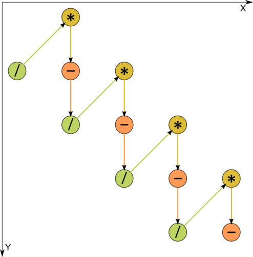
Figure 1. Graph of the algorithm. The input and output data are not shown. / - division, * - multiplication, - - subtraction.
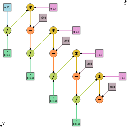
Figure 2. Graph of the algorithm. The input data are shown. / - division, * - multiplication, - - subtraction.


One can see from Figure 1, where one of the operations is decomposed into two constituents, that the information graph is purely serial.
1.8 Parallelization resource of the algorithm
In order to factorize a tri-diagonal matrix of order n by using the compact scheme of Gaussian elimination, one should perform
- [math]n-1[/math] layers of division,
- [math]n-1[/math] layers of multiplication,
- [math]n-1[/math] layers of addition (subtraction).
Each layer consists of a single operation. Hence, in terms of the parallel form height, the compact scheme of Gaussian elimination for factoring tri-diagonal matrices, in its serial version, is a linear complexity algorithm. The layer width is everywhere equal to 1. Thus, the entire algorithm is an all-over bottleneck.
1.9 Input and output data of the algorithm
Input data: tri-diagonal matrix [math]A[/math] (with entries [math]a_{ij}[/math]).
Size of the input data: [math]3n-2[/math]. Different implementations may store the information differently for economy reasons. For instance, each diagonal of the matrix can be stored by a separate row of the array.
Output data: lower bi-diagonal matrix [math]L[/math] (with entries [math]l_{ij}[/math], where [math]l_{ii}=1[/math]) and upper bi-diagonal matrix [math]U[/math] (with entries [math]u_{ij}[/math]).
Size of the output data is formally [math]3n-2[/math]. However, since [math]n[/math] items in the input and output data are identical, actually only [math]2n-2[/math] items are calculated.
1.10 Properties of the algorithm
It is clear that, in the case of unlimited resources, the ratio of the serial to parallel complexity is one (that is, the algorithm is non-parallelizable).
The computational power of the algorithm, understood as the ratio of the number of operations to the total size of the input and output data, is only a constant (the number of arithmetic operations is the same as the size of the data).
The algorithm is completely determined.
The equivalent perturbation [math]M[/math] of the algorithm does not exceed the perturbation [math]\delta A[/math] that results from inputting the data into memory: [math] ||M||_{E} \leq ||\delta A||_{E} [/math]
2 Software implementation of the algorithm
2.1 Implementation peculiarities of the serial algorithm
In its simplest version, the algorithm can be written in Fortran as follows:
	DO  I = 1, N-1
		A(I+1,I) = A(I+1,I)/A(I,I)
                A(I+1,I+1) = A(I+1,I+1) - A(I+1,I)*A(I,I+1)
	END DO
The decomposition is stored at the place where the original matrix was stored. The indexing is the same as for a dense matrix.
However, much more often, more economical schemes are used for storing tri-diagonal matrices. For instance, assume that the diagonals are numbered from left to right and each diagonal is stored by a separate row of the array. Then the following version is obtained:
	DO  I = 1, N-1
		A(1,I) = A(1,I)/A(2,I)
                A(2,I+1) = A(2,I+1) - A(1,I)*A(3,I)
	END DO
Here, the decomposition also overrides the original data. Under this storage scheme, the entries A(1,N) and A(3,N) are not addressed.
2.2 Locality of data and computations
The above program fragments show that the degree of locality of data and computations is very high. This is especially so for the second version in which all the data (both those needed by the current operation and the ones that it calculates) are stored and used nearby. However, the benefit from this high locality is limited by the fact that each computed item is afterwards used only once. The reason is simple: as already noted above, the size of the data processed by the algorithm is equal to the number of arithmetic operations.
2.3 Possible methods and considerations for parallel implementation of the algorithm
The compact scheme of Gaussian elimination as applied to the decomposition of tri-diagonal matrices is purely serial algorithm. It cannot be parallelized because each operation needs the result of the preceding one as an input and, in turn, passes its own result as the input of the next operation.
There exist variants of the parallelization of the compact scheme of Gaussian elimination for tri-diagonal matrices using the associativity of operations. Consequently, they represent entirely different algorithms that can be learned about at the corresponding page.
Furthermore, the possible case is where numerous decompositions of various tri-diagonal matrices are required. Then the above serial algorithm can be performed in parallel on different nodes of the computer system, each node processing its own matrix.
2.4 Scalability of the algorithm and its implementations
Since the algorithm is purely serial, the parallelization resource is completely lacking. It makes more sense to conduct all the calculations on a single processor.
2.5 Dynamic characteristics and efficiency of the algorithm implementation
2.6 Conclusions for different classes of computer architecture
Because of its serial structure, the algorithm, if not modified, can be efficiently implemented only on a computer of the classical Von Neumann architecture.