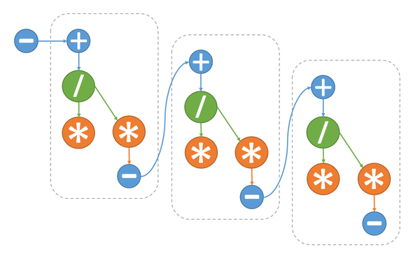
One step of the dqds algorithm

Алгоритм dqds нахождения сингулярных чисел двухдиагональной матрицы
Sequential algorithm
Serial complexity	[math]5n-4[/math]
Input data	[math]2n[/math]
Output data	[math]2n[/math]
Parallel algorithm
Parallel form height	[math]4n-3[/math]
Parallel form width	[math]2[/math]

Primary authors of this description: A.Yu.Chernyavskiy

1 Properties and structure of the algorithm

1.1 General description of the algorithm

The dqds algorithm iteration implements one step of the dqds algorithm for calculating the singular values of a bi-diagonal matrix.

The full dqds algorithm (differential quotient-difference algorithm with shifts) constructs a sequence of bi-diagonal matrices that converges to a diagonal matrix containing the squares of the required singular values. It has the merit of calculating the singular values to high accuracy.

The computational kernel of the algorithm is its inner iteration. Outside of the iterations, shifts [math]\delta[/math] (iteration parameters, see mathematical description of the algorithm) are chosen, convergence is looked after, and various optimization tricks are applied. Note that the non-iterative part of the algorithm is not important with respect to the structure of calculations because the main computational costs fall on the calculations within the iterations. Details concerning the non-iterative part, its variants, and the analysis of convergence can be found in the related literature .

1.2 Mathematical description of the algorithm

1.2.1 Auxiliary information

In order to understand the mathematical background of dqds iteration, it is helpful to briefly discuss its derivation, which, to same extent, reflects the history of the algorithm (the details can be found in ). It is convenient to begin with the so-called LR iteration, which predates the well-known QR iteration. Starting from the initial symmetric positive definite matrix [math]T_0\gt [/math], the LR algorithm constructs a converging sequence of matrices [math]T_i\gt 0[/math] that are similar to [math]T_0[/math]. In this construction, the following three steps are used iteratively:

1. Choose a shift [math]\tau_i[/math] that is less than the smallest eigenvalue of the matrix [math]T_i.[/math]
2. Compute the Cholesky decomposition [math]T_i-\tau^2_iI=B_i^TB_i,[/math] where [math]B_i[/math] is an upper triangular matrix with a positive diagonal.
3. [math]T_{i+1}=B_iB_i^T+\tau_i^2I.[/math]

Note that two steps of LR iteration with a zero shift are equivalent to a single step of QR iteration. This iterative procedure brings the matrix to diagonal form, calculating thereby the eigenvalues of the original matrix. It is easy to reformulate the LR algorithm for the problem of calculating the singular values of bi-diagonal matrices, and, for this problem, the algorithm becomes noticeably simpler. Namely, let us calculate a sequence of bi-diagonal matrices [math]B_i[/math] avoiding a direct calculation of matrices [math]T_i[/math] (which, in this case, are tri-diagonal). Let [math]B_i[/math] have the diagonal entries [math]a_1 \ldots a_n[/math] and the super-diagonal entries [math]b_1 \ldots b_{n-1}[/math], while [math]B_{i+1}[/math] has the diagonal entries [math]\widehat{a}_1 \ldots \widehat{a}_n[/math] and the super-diagonal entries [math]\widehat{b}_1 \ldots \widehat{b}_{n-1}.[/math] Then, in terms of the matrices [math]B_i[/math], one step of LR iteration can be reduced to a simple loop over [math]j[/math] running from [math]1[/math] to [math]n-1:[/math]

[math] \widehat{a}^2_j = a^2_j+b^2_j-\widehat{b}^2_{j-1}-\delta [/math]

[math] \widehat{b}^2_j = b^2_j\dot (a^2_{j+1}/a^2_j), [/math]

which is completed by the calculation of [math]\widehat{a}^2_n = a^2_n-\widehat{b}^2_{n-1}-\delta.[/math] The extraction of square roots is obviously better to postpone until the algorithm terminates; hence, one can set [math]q_j=a^2_j,\; e_j=b^2,[/math] which ultimately yields the so-called qds algorithm. It is given by the following formulas:

[math] \widehat{q}_j = q_j + e_j - \widehat{e}_{j-1} - \delta, \quad j \in [1,n-1] [/math]

[math] \widehat{e}_j = e_j \cdot q_{j+1} / \widehat{q}_j, \quad j \in [1,n-1] [/math]

[math] \widehat{q}_n = q_n - \widehat{e}_{n-1} - \delta. [/math]

Here, </math> [math]q_j, \; j \in [1,n][/math] and [math]e_j, \; j \in [1,n-1][/math] are the squares of the diagonal and super-diagonal entries, respectively. The circumflexes mark the output variables, and the symbol [math]\delta[/math] denotes the shift (which is a parameter of the algorithm). This is the most compact formulation of the so-called qds iteration.

1.2.2 Mathematical description of dqds iteration

Let us give the mathematical formulation of dqds iteration (from a mathematical viewpoint, qds and dqds iterations are equivalent), using the auxiliary variables [math]t_j[/math] and [math]d_j.[/math] One dqds iteration transforms the input bi-diagonal matrix [math]B[/math] to the output matrix [math]\widehat{B}.[/math]

Input and output data: [math]q_{j}, \; j\in [1,n], \; e_{k}, \; k\in [1,n-1] [/math] are the squares of the diagonal and super-diagonal entries of the input matrix [math]B[/math]; [math] \widehat{q}_j , \; \widehat{e}_k [/math] have the same meaning for the matrix [math]\widehat{B}[/math] to be calculated.

The method is given by the following formulas:

[math] d_1 = q_1 - \delta, \; q_n = d_n [/math]

для[math] \quad j\in [1,n-1]: [/math]

[math] \widehat{q}_j = d_j + e_j [/math]

[math] t_j = q_{j+1}/\widehat{q}_j [/math]

[math] \widehat{e}_j=e_j \cdot t_j [/math]

[math] d_{j+1} = d \cdot t - \delta [/math]

1.3 Computational kernel of the algorithm

The computational kernel of the algorithm consists in the successive calculation of the squares of the diagonal ([math]\widehat{q}_j[/math]) and super-diagonal ([math]\widehat{e}_k[/math]) entries of the output matrix. In view of the use of auxiliary variables, the calculation of each new pair requires one addition, one subtraction, one division, and two multiplications.

1.4 Macro structure of the algorithm

The algorithm consists of the separate calculation of the initial value of the auxiliary variable [math]d[/math], the subsequent execution (repeated (n-1) times) of the sequence of 5 operations (+,/,*,*,-) for calculating the squares of the diagonal ([math]\widehat{q}_j[/math]) and super-diagonal ([math]\widehat{e}_k[/math]) entries of the output matrix, and the concluding calculation of the last value [math]\widehat{q}_n[/math].

1.5 Implementation scheme of the serial algorithm

Note that the output data can right away be written to the locations of the old data (which is used in the scheme). To store the auxiliary variables [math]t_j[/math] and [math]d_j[/math], it is sufficient to have two rewritable variables. Thus, the diagonal ([math]q_j[/math]) and super-diagonal ([math]e_k[/math]) entries of the input matrix are successively replaced by the corresponding entries of the output matrix.

The operations in the method are performed in the following order:

1. Compute the initial value of the auxiliary variable [math]d = q_1-\delta.[/math]

2. Perform a loop over j from 1 to n-1. It consists of the following:

2.1 Compute the value [math]q_j = d + e_j;[/math]

2.2 Compute the value of the auxiliary variable [math]t = q_{j+1}/q_j;[/math]

2.3 Compute the value [math]e_j = e_j \cdot t;[/math]

2.4 Compute the value of the auxiliary variable [math]d = d \cdot t - \delta.[/math]

3. Compute [math]q_n = d.[/math]

These calculations can be organized in a different form, for instance, in the form of qds iteration (see Mathematical description of dqds iteration). However, it is dqds implementation that makes it possible to attain high accuracy .

1.6 Serial complexity of the algorithm

In order to perform one dqds iteration, it is necessary to execute

• [math]n-1[/math] divisions,
• [math]2n-2[/math] multiplications,
• [math]2n-1[/math] additions/subtractions.

Thus, one dqds iteration has a linear complexity.

1.7 Information graph

Figure 1. The algorithm graph for n=4. The input and output data are not shown.

1.8 Parallelization resource of the algorithm

The information graph of the algorithm shows that, at each step of the main loop, only multiplication (2.2) and multiplication + addition (2.4) can be executed in parallel. This makes it possible to reduce the number of layers per loop iteration from 5 to 4 and the overall number of layers in the algorithm from 5n-4 to 4n-3. The layers with multiplications contain two operations, while the other layers contain only one operation.

1.9 Input and output data of the algorithm

Input data: The squares of the diagonal and super-diagonal entries of the input bi-diagonal matrix (the vector [math]q[/math] of length n and the vector [math]e[/math] of length n-1) and the shift parameter [math]\delta[/math].

Size of the input data: [math]2n[/math].

Output data: The squares of the diagonal and super-diagonal entries of the output bi-diagonal matrix.

Size of the output data: [math]2n-1[/math].

1.10 Properties of the algorithm

If the parallel execution of multiplications is possible, then the ratio of the serial to parallel complexity is [math]\frac{5n-4}{4n-3}[/math], that is, the algorithm is poorly parallelizable.

The computational power of the algorithm, understood as the ratio of the number of operations to the total size of the input and output data, is a constant.

The algorithm is completely determined.

2 Software implementation of the algorithm

2.1 Implementation peculiarities of the serial algorithm

In the Matlab language, the algorithm can be written as follows:

d = q(1)-delta;
for j = 1:n-1
    q(j)=d+e(j);
    t=q(j+1)/q(j);
    e(j) = e(j)*t;
    d = d*t-delta;
end
q(n) = d;

As already said in the section Implementation scheme of the serial algorithm, the calculated values are written to the locations of the input data.

2.2 Locality of data and computations

It is easy to see that the data locality is high. It can be further improved by placing alongside the corresponding elements of the arrays e и q. However, this does not significantly affect the algorithm performance because the ratio of the number of operations to the number of processed data is a constant.

2.2.1 Locality of implementation

2.2.1.1 Structure of memory access and a qualitative estimation of locality

Figure 2. The dqds algorithm iteration. Overall memory address profile.

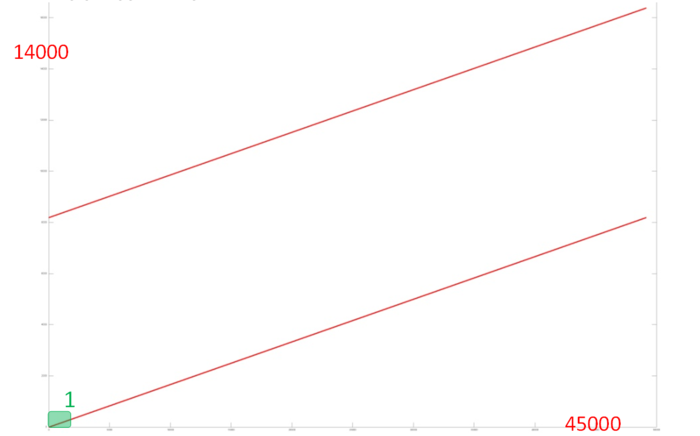
Fig.2 shows the memory address profile for one iteration of the dqds algorithm. In outward appearance, this profile has a very simple structure and consists of two serial searches performed in parallel. Notice that the overall number of memory accesses is only 3 times larger than the number of processed data. This says that the data are rarely used repeatedly, which often indicates that locality is rather poor.

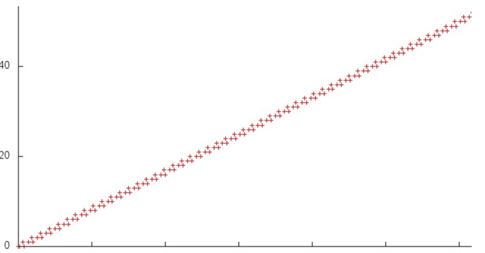
Consider the structure of one search in more detail (the structure of the other search is practically the same). Fig.3 shows the small fragment 1 of Fig. 2. One can see that three memory accesses are performed at each step of the search. This indicates a high spatial locality; however, the temporal locality is low the data are used only 3 times.

Since this structure of accesses is inherent in the overall profile, the above observations are also valid for its locality.

Figure 3. The address profile, fragment 1

2.2.1.2 Quantitative estimation of locality

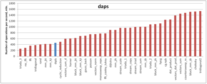
The estimate is based on daps, which assesses the number of memory access operations (reads and writes) per second. Similarly to flops, daps is used to evaluate memory access performance rather than locality. Yet, it is a good source of information, particularly for comparison with the results provided by the next estimate cvg.

Figure 4 shows the daps values for implementations of certain popular algorithms. These values are sorted in ascending order (the greater the daps, the higher the performance in general). The result is fairly unexpected, namely, the memory performance is very low. The daps estimate for this profile is comparable with those for algorithms that are most inefficient as regards memory performance such as the RandomAccess tests and inefficient variants of the conventional matrix multiplication. To some extent, this can be explained by the low temporal locality. However, here, there is another possible reason. For this implementation, the volume of computations per memory access is sufficiently large, which may cause the memory underload. In this case, performance is rather low despite the fact that the efficiency of memory interaction is on the whole not bad.

Figure 4. Comparison of daps values

2.3 Possible methods and considerations for parallel implementation of the algorithm

The dqds iteration is practically entirely serial. The only possibility for parallelization is the simultaneous execution of multiplication (2.2) and multiplication + addition (2.4), which yields a small gain in performance.

2.4 Scalability of the algorithm and its implementations

The algorithm is not scalable. The maximum acceleration is attained for two independent processors.

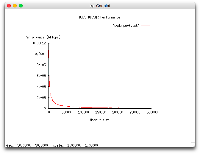
Let us study this implementation as regards scaling out in accordance with Scalability methodology. This study was conducted using the Lomonosov-2 supercomputer of the Moscow University Supercomputing Center.

Variable parameters for the launch of the algorithm implementation and the limits of parameter variations:

• number of processors 1;
• matrix size [1000 : 260000] with the step 500.

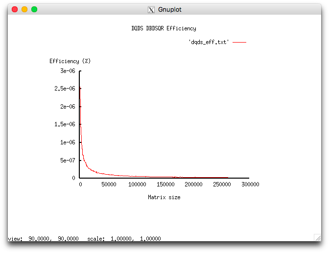
The experiments resulted in the following range of implementation efficiency:

• minimum implementation efficiency 2.559e-06%;
• maximum implementation efficiency 2.492e-08%.

The following figures show the graphs of the performance and efficiency for the chosen implementation of DQDS as functions of the variable launch parameters.

Figure 8. Parallel implementation of dqds algorithm. Performance as a function of the number of processors and the matrix size.

Figure 9. Parallel implementation of dqds algorithm. Efficiency as a function of the number of processors and the matrix size.

Study of the parallel implementation in the C language

2.6 Conclusions for different classes of computer architecture

An efficient implementation of the algorithm is only possible on a computer facility with one core or two.

2.7 Existing implementations of the algorithm

Сам алгоритм dqds реализован в функции xBDSQR пакета LAPACK и используется при её вызове без расчёта сингулярных векторов.