Backward substitution

Backward substitution
Sequential algorithm
Serial complexity	[math]O(n^2)[/math]
Input data	[math]O(n^2)[/math]
Output data	[math]n[/math]
Parallel algorithm
Parallel form height	[math]O(n)[/math]
Parallel form width	[math]O(n)[/math]

Primary authors of this description: A.V.Frolov, Vad.V.Voevodin (Section 2.2), A.M.Teplov (Section 2.4)

1 Properties and structure of the algorithm

1.1 General description of the algorithm

Backward substitution is a procedure of solving a system of linear algebraic equations [math]Ux = y[/math], where [math]U[/math] is an upper triangular matrix whose diagonal elements are not equal to zero. The matrix [math]U[/math] can be a factor of another matrix [math]A[/math] in its decomposition (or factorization) [math]LU[/math], where [math]L[/math] is a lower triangular matrix. This decomposition can be obtained by many methods (for example, the Gaussian elimination method with or without pivoting, the Gaussian compact scheme, the Cholesky decomposition, etc.). Here we also should mention the [math]QR[/math] decomposition when the matrix [math]A[/math] is represented in the form [math]A=QR[/math], where [math]Q[/math] is an orthogonal matrix and [math]R[/math] is an upper triangular matrix. Since the matrix [math]U[/math] is triangular, a procedure of solving a linear system with the matrix [math]U[/math] is a modification of the general substitution method and can be written using simple formulas.

A similar procedure of solving a linear system with a lower triangular matrix is called the forward substitution (see). Note that the backward substitution discussed here can be considered as a part of the backward Gaussian elimination in the Gaussian elimination method for solving linear systems.

There exists a similar method called the backward substitution with normalization. The scheme of this modification is more complex, since a number of special operations are performed to reduce the effect of round-off errors on the results. This modified method is not discussed here.

1.2 Mathematical description of the algorithm

Input data: an upper triangular matrix [math]U[/math] whose elements are denoted by [math]u_{ij}[/math]); a right-hand vector [math]y[/math] whose components are denoted by [math]y_{i}[/math]).

Output data: the solution vector [math]x[/math] whose components are denoted by [math]x_{i}[/math]).

The backward substitution algorithm can be represented as

[math] \begin{align} x_{n} & = y_{n}/u_{nn} \\ x_{i} & = \left (y_{i} - \sum_{j = i+1}^{n} u_{ij} x_{j} \right ) / u_{ii}, \quad i \in [1, n - 1]. \end{align} [/math]

There exists a block version of this algorithm; however, here we consider only its “dot” version.

1.3 Computational kernel of the algorithm

The computational kernel of the backward substitution algorithm can be composed of [math]n-1[/math] dot products of subrows of the matrix [math]U[/math] with the computed part of the vector [math]x[/math]:

[math] \sum_{j = i+1}^{n} u_{ij} x_{j} [/math].

Here the dot products can be accumulated in double precision for additional accuracy. These dot products are subtracted from the components of the vector [math]y[/math] and the results are divided by the diagonal elements of the matrix [math]U[/math]. In some implementations, however, this approach is not used. In these implementations, the operation

[math] y_{i} - \sum_{j = i+1}^{n} u_{ij} x_{j} [/math]

is performed by subtracting the componentwise products as part of dot products from [math]y_{i}[/math] instead of subtracting the entire dot product from [math]y_{i}[/math]. Hence, the operation

[math] y_{i} - \sum_{j = i+1}^{n} u_{ij} x_{j} [/math]

and the division of the results by the diagonal elements of the matrix should be considered as a computational kernel instead of the dot product operations. Here the accumulation in double precision can also be used.

1.4 Macro structure of the algorithm

As is stated in description of algorithm’s kernel, the major part of the algorithm consists of computing the ([math]n-1[/math]) sums

[math]y_{i} - \sum_{j = i+1}^{n} u_{ij} x_{j} [/math]

and dividing the results by the diagonal elements of the matrix. The accumulation in double precision can also be used.

1.5 Implementation scheme of the serial algorithm

The first stage of this scheme can be represented as

1. [math]x_{n} = y_{n}/u_{nn}[/math].

At the second stage, for all [math]i[/math] form [math]n-1[/math] to [math]1[/math], the following operations should be performed:

2. [math]x_{i} = \left (y_{i} - \sum_{j = i+1}^{n} u_{ij} x_{j} \right ) / u_{ii}[/math].

Note that the computations of the sums [math]y_{i} - \sum_{j = i+1}^{n} u_{ij} x_{j}[/math] are performed in the accumulation mode by subtracting the products [math]u_{ij} x_{j}[/math] from [math]y_{i}[/math] for [math]j[/math] from [math]n[/math] to [math]i + 1[/math] with decreasing [math]j[/math]. Other orders of summation lead to a severe degradation of parallel properties of the algorithm. As an example, we can mention a program fragment given in, where the backward substitution is discussed in the form of the backward Gaussian elimination performed with increasing summation index because of the restrictions imposed by old versions of Fortran.

1.6 Serial complexity of the algorithm

The following number of operations should be performed for the backward substitution in the case of solving a linear system with an upper triangular matrix of order [math]n[/math] using a serial most fast algorithm:

• [math]n[/math] divisions
• [math]\frac{n^2-n}{2}[/math] additions (subtractions),
• [math]\frac{n^2-n}{2}[/math] multiplications.

The main amount of computational work consists of multiplications and .additions (subtractions)

In the accumulation mode, the multiplication and subtraction operations should be made in double precision (or by using the corresponding function, like the DPROD function in Fortran), which increases the overall computation time of the algorithm.

Thus, the computational complexity of the backward substitution algorithm is equal to [math]O(n^2)[/math].

1.7 Information graph

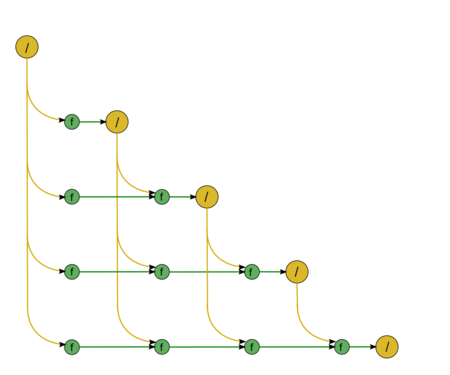
Let us describe the algorithm’s graph analytically and in the form of a figure. The graph of the backward substitution algorithm]consists of two groups of vertices positioned in the integer-valued nodes of two domains of different dimension.

Figure 1. Backward substitution.

The first group of vertices belongs to the one-dimensional domain corresponding to the division operation. The only coordinate [math]i[/math] of each vertex changes in the range from [math]n[/math] to [math]1[/math] and takes all the integer values from this range.

The dividend of this division operation:

• for [math]i = n[/math]: the input data element [math]y_{n}[/math];
• for [math]i \lt n[/math]: the result of the operation corresponding to the vertex of the second group with coordinates [math]i[/math], [math]i+1[/math].

The divisor of this division operation is the input data element [math]u_{nn}[/math].

The result of this operation is the output data element [math]x_{i}[/math].

The second group of vertices belongs to the two-dimensional domain corresponding to the operation [math]a-bc[/math].

The coordinates of this domain are as follows:

• the coordinate [math]i[/math] changes in the range from [math]n-1[/math] to [math]1[/math] and takes all the integer values from this range;
• the coordinate [math]j[/math] changes in the range from [math]n[/math] to [math]i+1[/math] and takes all the integer values from this range.

The arguments of this operation:

• [math]a[/math]:
  • for [math]j = n[/math]: the input data element [math]y_{i}[/math];
  • for [math]j \lt n[/math]: the result of the operation corresponding to the vertex of the second group with coordinates [math]i, j+1[/math];
• [math]b[/math]: the input data element [math]u_{ij}[/math];
• [math]c[/math]: the result of the operation corresponding to the vertex of the first group with coordinate [math]j[/math];

The result of this operation is intermediate for the backward substitution algorithm.

The above graph is illustrated in Fig. 1 for [math]n = 5[/math]. In this figure, the vertices of the first group are highlighted in yellow and are marked by the division sign; the vertices of the second group are highlighted in green and are marked by the letter f. The graph shows the input data transfer from the vector [math]y[/math], whereas the transfer of the matrix elements [math]u_{ij}[/math] to the vertices is not shown.

1.8 Parallelization resource of the algorithm

In order to implement the backward substitution algorithm for a linear system with an upper triangular matrix of order [math]n[/math], a parallel version of this algorithm should perform the following layers of operations:

• [math]n[/math] layers of divisions (one division on each of the layers),
• [math]n - 1[/math] layers of multiplications and [math]n - 1[/math] layers of addition/subtraction (on each of the layers, the number of these operations is linear and varies from [math]1[/math] to [math]n-1[/math].

Contrary to a serial version, in a parallel version the division operations require a significant part of overall computational time. The existence of isolated divisions on some layers of the parallel form may cause other difficulties for particular parallel computing architectures. In the case of programmable logic devices (PLD), for example, the operations of multiplication and addition/subtraction can be conveyorized, which is efficient in resource saving for programmable boards, whereas the isolated division operations acquire resources of such boards and force them to be out of action for a significant period of time.

In addition, we should mention the fact that the accumulation mode requires multiplications and subtraction in double precision. In a parallel version, this means that almost all intermediate computations should be performed with data given in their double precision format. Contrary to a serial version, hence, the amount of the necessary memory increases to some extent.

Thus, the backward substitution algorithm belongs to the class of algorithms of linear complexity in the sense of the height of its parallel form; its complexity is also linear in the sense of the width of its parallel form.

1.9 Input and output data of the algorithm

Input data: an upper triangular matrix [math]U[/math] of order [math]n[/math] whose elements are denoted by [math]u_{ij}[/math] and the right-hand side vector [math]y[/math] whose components are denoted by [math]y_{i}[/math]).

Amount of input data: :[math]\frac{n (n + 3)}{2}[/math]; since the matrix is triangular, it is sufficient to store only the nonzero elements of the matrix [math]U[/math]).

Output data: the solution vector [math]x[/math] whose components are denoted by [math]x_{i}[/math]).

Amount of output data: [math]n[/math].

1.10 Properties of the algorithm

In the case of unlimited computer resources, the ratio of the serial complexity to the parallel complexity is linear (the ratio of quadratic complexity to linear complexity).

The computational power of the Cholesky algorithm considered as the ratio of the number of operations to the amount of input and output data is only a constant.

The backward substitution algorithm is completely deterministic. Another order of associative operations is not considered for this algorithm’s version under study, since in this case the structure of the algorithm radically changes and the parallel complexity becomes quadratic.

The linear number of the parallel form layers consisting of a single division slows the performance of the parallel version and is a bottleneck of the algorithm, especially compared to the forward substitution, where the diagonal elements are equal to 1. In this connection, when solving linear systems, it is preferable to use the triangular decompositions for which the triangular factors contain the diagonals whose elements are equal to 1. When such triangular factors are nonsingular, it is useful, before solving the linear system, to transform them the product of a diagonal matrix and a triangular matrix whose diagonal elements are equal to 1.

There exist several block versions of the backward substitution algorithm. The graphs of some of them are almost coincident with the graph of the dot version; the distinctions consist in the ways of unrolling the loops and their rearrangements. Such an approach is useful to optimize the data exchange for particular parallel computing systems.

2 Software implementation of the algorithm

2.1 Implementation peculiarities of the serial algorithm

In its simplest version, the backward substitution algorithm can be represented in Fortran as

        X(N) = Y(N) / U (N, N)
	DO  I = N-1, 1, -1
		S = Y(I)
		DO  J = N, I+1, -1
			S = S - DPROD(U(I,J), X(J))
		END DO
		X(I) = S / U(I,I)		
	END DO

Here [math]S[/math] is a double precision variable if the accumulation mode is used.

2.2 Locality of data and computations

2.2.1 Locality of implementation

2.2.1.1 Structure of memory access and a qualitative estimation of locality

Figure 2. The backward Gaussian elimination. A general memory-access profile.

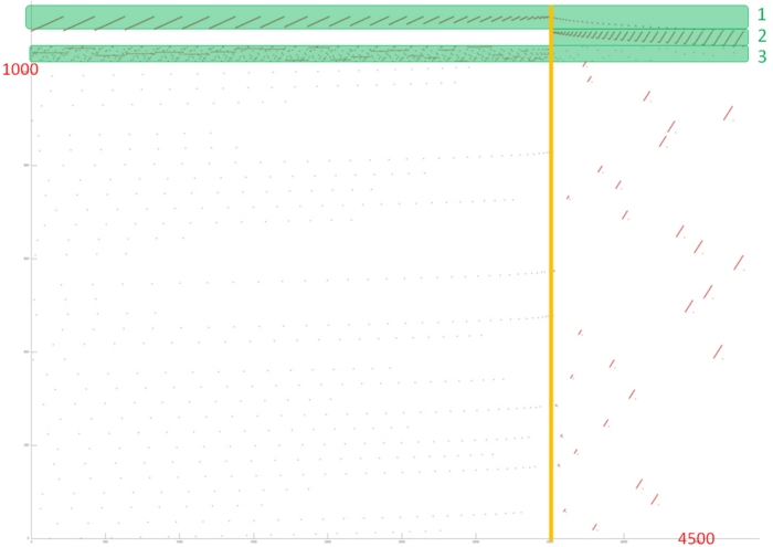
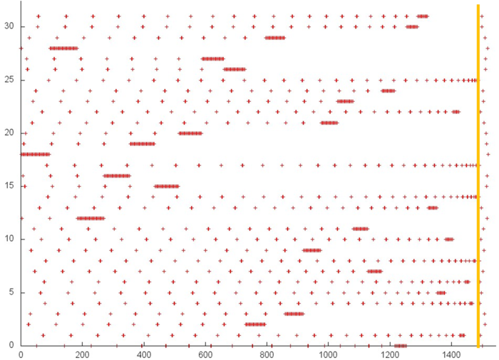
Fig.2 illustrates a general memory-access profile for an implementation chosen to study the backward Gaussian elimination. From this figure it follows that this profile consists of two stages (the boundary between them is highlighted in orange). These stages correspond to the two loops of this implementation taken for our analysis. Based on this analysis, we conclude that the memory-access profile consists of the references to 4 arrays. In Fig. 2, three of them are highlighted in green; the other references are made to the fourth array. Note that the total number of references is greater only by several times than the number of the used elements (4500 and 1000, respectively). Hence, it is difficult to achieve a high degree of locality.

In order to clarify this situation, we consider each of these arrays individually.

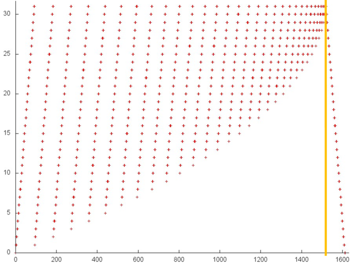
Fig.3 illustrates fragment 1. The orange line delimits the above two stages. The second stage is a linear search in the reverse order. The first stage is iterative: at each iteration, the array’s element with the smallest number is dropped. Such a profile is characterized by a high spatial locality, since the elements are searched in succession, and by a sufficiently high temporal locality, since the repeated references are made to the same elements at each iteration.

Figure 3. Fragment 1 (the profile of references to the first array).

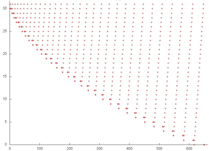
Fig.4 illustrates fragment 2 corresponding to the references to the second array. This fragment is smaller than the previous one: only 600 memory references. In essence, this fragment is similar to fragment 1 (Fig. 3), the only distinction consists in the fact that the iterations are performed in the reverse order. However, this distinction has a little effect on the spatial locality and on the temporal locality. Hence, fragment 2 possesses the same properties.

Figure 4. Fragment 2 (the profile of references to the second array).

Fig.5 illustrates fragment 3. The orange line also delimits the above two stages. A small number of references are made at the second stage. The references of the first stage are similar to a random access occurring frequently in the case of indirect addressing. Sometimes, many references are made to a certain element in succession, but after that this element is no more used. Usually, such a profile is characterized by a low spatial and temporal locality; however, this disadvantage is not so important, since the number of the element in use is small.

Figure 5. Fragment 3 (the profile of references to the third array).

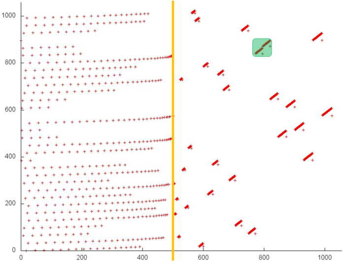
Now we consider the fragment occupying the major part of Fig.2. This profile is presented in Fig.6. The following peculiarity of this profile should be mentioned: more than 1000 elements are used, whereas about 30 elements are used in the other profiles. The number of references is less than the number of references to the first and third arrays.

It should also be noted that the major part of references are made at the second stage. The first stage is similar to the first stage of the previous array (Fig.5); the only exception consists in the fact that in this profile there no multiple references in succession to a single element before this element is no more used. The first stage consists of about 500 references distributed uniformly on a segment of 1000 elements; hence, a very low spatial and temporal locality is observed.

At the second stage, the references are of another character. This stage possesses a higher spatial locality, since the references are grouped in clusters whose structures are similar. However, the structure of the cluster itself requires a deeper analysis.

Figure 6. Fragment 4 (the profile of references to the fourth array).

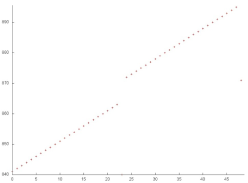
Figure 7 illustrates the two clusters highlighted in green in Fig.6. The scale of Fig.7 allows one to see that each cluster is a linear search with a small step in a subset of the array elements.

Hence, we can conclude that the second stage of fragment 4 possesses a sufficiently high spatial locality, since each cluster contains linear search operations, but the temporal locality is low, since the repeated references are almost absent.

Figure 7. Two clusters from fragment 4.

The following conclusion can be made for the entire profile: the first three arrays (especially, the first and second arrays) have a sufficiently high locality. However, a rather low spatial locality and a very low temporal locality of the fourth array significantly reduce the general locality of the entire implementation under study.

2.2.1.2 Quantitative estimation of locality

The main fragment of the implementation used to obtain the quantitative estimates is given here (the Kernel2 function). The start conditions are discussed here.

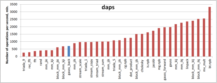
The first estimate is made on the basis of the daps characteristic used to evaluate the number of write and read operations per second. This characteristic is similar to the flops estimate for memory access and is an estimate of the memory usage performance rather than an estimate of locality. However, the daps characteristic is a good information source and can be used to compare with the results obtained according to the cvg characteristic.

Fig.8 illustrates the daps values for a number of some widespread algorithms. These values are given in increasing order: a higher performance corresponds to a larger daps value. From this figure it follows that , according to our above discussion about a negative effect of one of the arrays, this implementation is characterized by a low memory usage performance compared to the forward Gaussian elimination.

Figure 8. Comparison of daps values.

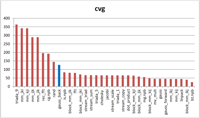
The cvg characteristic is used to obtain a more machine-independent estimate of locality and to specify the frequency of fetching data to the cache memory. A lesser cvg value corresponds to a higher level of locality and to a smaller number of using the fetching procedure.

Fig.9 shows the cvg values for the same implementations presented in Fig. 8. These values are given in decreasing order: a higher locality level corresponds to a smaller cvg value. From this figure it follows that, according to the cvg estimate, the memory access profile possesses a low locality, but a little bit better than in the case of random memory access. This conclusion is similar to that based on our analysis of the daps characteristic.

Figure 9. Comparison of cvg values.

2.3 Approaches and features of implementing the back substitution algorithm in parallel

There are not so many possibilities to implement the back substitution algorithm in parallel. Both of the main loops of this algorithm can be unrolled and, hence, its block version can be considered. The algorithm’s versions without unrolling the loops are possible using the completely parallel loops over I:

        DO  PARALLEL I = 1, N
           X(I) = Y(I)
        END DO
        DO J = N, 1, -1
           X(J) = X(J) / U(J,J)
           DO PARALLEL I = 1, J-1
              X(I) = X(I) - U(I,J)*X(J)
           END DO
        END DO

It is also possible to use the "skewed parallelism" in the above loops.

2.6 Conclusions for different classes of computer architecture

Based on the analysis of the algorithm’s structure, we can conclude that, in order to minimize the data exchange between computing nodes, we should choose a block version such that all the matrix elements are accessible on all nodes or are distributed on the nodes in advance. In this case the amount of data transferred between the nodes is small compared to the number of arithmetic operations. In this approach, however, the largest reduction of performance efficiency is caused by the nonoptimality of computations within individual blocks. Hence, it is necessary to first optimize not an entire algorithm but the subroutines used on individual processors, such as the dot backward substitution algorithm, matrix multiplications, etc. A number of possible directions of such an optimization are discussed below.

2.7 Existing implementations of the algorithm

The real-valued version of the backward substitution algorithm is implemented in the basic libraries produced in Russia and in the libraries produced in western countries (for example, in LINPACK, LAPACK, ScaLAPACK, and others).

In the Russian libraries, as a rule, the accumulation mode is implemented to reduce the effect of round-off errors. In the modern western libraries, the dot versions of the algorithm are based on its LINPACK implementation utilizing the BLAS package.

In the majority of libraries, there exists a block version of the backward substitution algorithm such that its graph is topologically identical to the graph of its dot version. Since the amount of transferred data is approximately equal to the number of arithmetic operations, the optimal usage of caches in the block versions can increase their performance. Hence, an optimization of caching should first be done to optimize the performance of algorithm’s implementations.